BIN-SX-Chimera

UCSF Chimera: Structure Visualization and Analysis

Keywords: UCSF Chimera; Structure visualization; Structure analysis

Caution!

This unit is under development. There is some contents here but it is incomplete and/or may change significantly: links may lead to nowhere, the contents is likely going to be rearranged, and objectives, deliverables etc. may be incomplete or missing. Do not work with this material until it is updated to "live" status.

Abstract

This unit introduces the molecular viewer UCSF Chimera, starts you off on a routine to practice stereo viewing of molecular models, and teaches how to use Chimera to solve a number of common visualization and analysis tasks.

This unit ...

Prerequisites

You need to complete the following units before beginning this one:

BIN-PDB (The RCSB-PDB Structure Database)

Objectives

This unit will ...

... introduce ;
... teach ;
... demonstrate .

Outcomes

After working through this unit you ...

... know what the most important terms of graph theory mean;
... are familar with a number of quantitiative measures on graphs;
... can use igraph to construct graphs, plot graphs with a variety of layout algorithms, and analyse their degree distribution, centrality distribution, and community structure;
... can interpret such measures in a biological context.

Deliverables

Time management: Before you begin, estimate how long it will take you to complete this unit. Then, record in your course journal: the number of hours you estimated, the number of hours you worked on the unit, and the amount of time that passed between start and completion of this unit.
Journal: Document your progress in your Course Journal. Some tasks may ask you to include specific items in your journal. Don't overlook these.
Insights: If you find something particularly noteworthy about this unit, make a note in your insights! page.

Evaluation

This learning unit can be evaluated for a maximum of 6 marks. If you want to submit tasks for this unit for credit you have the following options. If you have any questions about these options, discuss on the mailing list.

Short Report option: 1. Create a new page on the student Wiki as a subpage of your User Page.; 2. Alpha helices orient peptide carbonyls parallel to their axis and since the C=O bond is polarized with an excess of electrons near the carboyl oxygen, this creates an induced dipole along the length of the helix, with a positive partial charge towards the beginning of the helix, and a negative partial charge towards its end. To compensate, we often find negativeley charged residues at the beginning of the helix and positively charged residues at the end - to stabilize the helix. However, for DNA binding, electrostatic complementarity would make us assume that alpha helices in DNA binding proteins are generally oriented with the (+)-dipole close to the DNA phosphates, and that there are no compensating charged residues at the termini. Write a short analysis on one of the three following topics - A, B, or C. The goal of this short report is to connect visualization to biology.

A - Helix dipoles: Nucleosome core

A.1 Open Chimera and load the structure 5XF3.

A.2 Study the complex with respect to this assumption. Produce 2 or more informative stereo-images that illustrate your findings.

A.3 Write up, illustrate, and interpret your findings in a short report.

B - Helix dipole: Transcription factor

B.1 Open Chimera and load the structure 4Y60.

B.2 Study the complex with respect to this assumption. Produce 2 or more informative stereo-images that illustrate your findings.

B.3 Write up, illustrate and interpret your findings in a short report.

C - Helix dipole: Transcription factor

C.1 Open Chimera and load the structure 4ZSF.

C.2 Study the complex with respect to this assumption. Produce 2 or more informative stereo-images that illustrate your findings.

C.3 Write up, illustrate and interpret your findings in a short report.

3. When you are done with your report, add the following category tag to the page:

[[Category:Eval-SX-Chimera]]

Do not change your submission page after this tag has been added. The page will be marked and the category tag will be removed by the instructor.

Quizzes will be written in class, back-to-back if there is more than one quiz scheduled. We may begin at any time. We will have an open-ended Q&A session before the quiz. You can't take the quiz if you are not present in class when the question sheets are handed out, so don't be late. Once all scheduled quizzes are written, we will discuss and mark them. You will mark your own quiz. All marking must be done with a red pen - so you must bring a red pen to class in order to participate. The mark you give yourself may be revised by the instructor after spot-checking quizzes. If this is necessary, you will be notified. You must mark your quiz correctly and honestly - don't get into trouble with academic integrity rules: it will be an academic offence if you mark questions as correct that were discussed in class and should have been marked incorrect. When in doubt, ask.

-->

Option to write a protein structure gallery entry

Write a short section, modelled on the other sections in this unit that explores an aspect of using Chimera for visual analysis using the 1DP7 transcription factor/DNA complex if possible. Choose one of the following biological facts or topics; then eMail me for confirmation (so we don't have everyone working on the same option).

Biological facts (show one stereo-image image that illustrates the fact, explain the fact in the image caption, and write a step by step description how to create that image.)

Hydrophobic amino acids are concentrated in the core (show a slice through 1BM8, rendered with solid spheres, where amino acids are clored by hydrophobicity)
Proline residues are rare in alpha-helices (show a normal alpha helix, and how an alpha helix with a proline distorts the helix)
Some structures don't show the active "biological unit"
The crystal structure sits in a lattice of symmetry related molecules
Disordered loops are not included in the coordinates
NMR structures contain hydrogen atoms - X-ray structures do not
Trypsin and subtilisin contain similar catalytic triads in an unrelated structural context
Membrane spanning proteins often have a ring of tryptophan residues anchoring them to the membrane

Use of Chimera

Labels and distance monitors
Structure superposition (1DP7 and 1BM8)
Use of attributes to visually map protein properties to protein structure (cf. </small)

Write a step-by-step tutorial to create an illustration for the fact or explore the use of Chimera (stereo image!). (The Chimera "Image Tutorials" may provide inspiration about different types of images that are available.)
Create a new page on the student Wiki as a subpage of your User Page. Develop your tutorial there.
When you are done with developing this contents, add the following category tag to the page:

[[Category:EVAL-SX-Chimera]]

Do not change your submission page after this tag has been added. The page will be marked and the category tag will be removed by the instructor.

Molecular graphics: UCSF Chimera

To view molecular structures, we need a tool to visualize the three dimensional relationships of atoms. A molecular viewer is a program that takes 3D structure data and allows you to display and explore it. For a number of reasons, I use the UCSF Chimera viewer for this course:

Chimera is free and open;
It creates very appealing graphics;
It is under ongoing development and is well maintained (actually, Chimera's next generation version "ChimeraX" will be released soon);
It provides an array of useful utilities for structure analysis; and,
besides an intuitive, menu driven interface, Chimera can be scripted via its command line, or even programmed via its in-built python interpreter.

Chimera: First steps

Task:

Installation

Access the Chimera homepage and navigate to the Download section.
Find the the newest version for your platform in the table and click on the file to download it.
Follow the instructions to install Chimera.

First tutorial

The Chimera User Guide site has a set of associated tutorials and there are more tutorials linked from here.

Work through Part 1 and Part 2 of the "Getting Started" Tutorial

Stereo Viewing

Stereo viewing is easy to learn with a molecular viewer like Chimera.

Being able to visualize and experience structure in 3D is an essential skill if you are at all serious about understanding the molecules of molecular biology. This is not sufficiently realized in the field: many molecular biologists have never invested the effort it takes to learn the skill and thus will tell you that it is not actually necessary, and you can get by regardless. Of course you are talking to a biased population – unless you have experienced and worked with stereo images, you can't understand how much you are actually missing. But once you have acquired the skill, you'll regret not having been taught earlier. Speak to people who use stereo vision: seeing molecules in 3-D is like the difference between seeing a photograph of a place and actually being there. In 3D you can appreciate size, scale, distance, spatial relations all at a single glance. I insist: you can't understand structure unless you experience it in 3D.

From 2D to pseudo 3D
Images we see on screen or on paper are two-dimensional projections of three-dimensional objects.

Even though hardware devices exist that help in the three-dimensional perception of computer graphics images, for the serious structural biologist there is really no alternative to being able to fuse stereo pair images by looking at them. Chimera is an excellent tool to practice stereo viewing and develop the skill. Stereo images consist of a left-eye and a right-eye view of the same object, with a slight rotation around the vertical axis (about 5 degrees). Your brain can accurately calculate depth from these two images, if they are presented to the right and left eye separately. This means you need to look at the two images and then fuse them into a single image - this happens when the left eye looks directly at the left image and the right eye at the right image.

In this tutorial, I teach you a method to learn stereo viewing. The method is pretty foolproof - I have taught this many years in my classes with virtually 100% success rates. But I can only teach you the method – learning must be done by you.

Some people find convergent (cross-eyed) stereo viewing easier to learn. I recommend the divergent (wall-eyed) viewing - not only because it is much more comfortable in my experience, but also because it is the default way in which stereo images in books and manuscripts are presented. The method explained below will only work for learning to view divergent stereo pairs.

Physiology

In order to visually fuse stereo image pairs, you need to override a vision reflex that couples divergence and focusing. This needs to be practiced for a while. Usually 5 to 10 minutes of practice twice daily for a week should be quite sufficient. It is not as hard as learning to ride a bicycle, but you need to practice regularly for some time, maybe 10 or 20 sessions of 3 to 5 minute over a period of a week or two. Once you have acquired the skill, it is really very comfortable and can be done effortlessly and for extended periods. You will enter a new world of molecular wonders!

Practice

Task:
Here are step by step instructions of how to practice stereo viewing with Chimera.

Load the Mbp1 APSES domain structure 1BM8 small protein into Chimera and display it as a simple backbone model.
- Start Chimera.
- Select File→Fetch by ID... choose PDB, type 1BM8 in the form and click Fetch.
- Choose Presets → Publication 1 ..., and
- ... Tools → Viewing Controls → Effects: check depth cueing ON and shadows OFF; use the Side View menu to move the clipping planes close to your model.
- Apply a nice coloring ramp: Tools → Depiction → Rainbow and click Apply
Set the stereo display to view the scene as a side-by-side stereo pair:
- Tools → Viewing Controls → Camera and select camera mode: wall-eye stereo.

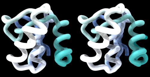
The model could look something like this:

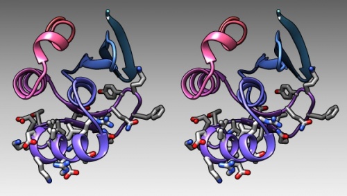
1BM8: Mbp1 transcription factor APSES domain rendered as a ribbon model, with depth-cueing applied and a colour-ramp emphasizing the fold from N-C terminus. The molecule is shown in wall-eye stereo: the left-hand image is rotated correctly for the left eye. You should resize the window of your molecular viewer (Chimera) until equivalent points are about 15% less than your pupil separation apart.

For the next step, you need to know how far your eyes are apart. Not just approximately, but pretty accurately. Measure the distance between your pupils in front of a mirror, or have soemone help you.
Resize the horizontal distance of the viewing window by dragging its lower right-hand corner. This changes the separation of the two views.
- Resize the window so that two equivalent points on the protein are about 15% closer together on the screen than the pupils of your eyes are apart. Calculate, and measure eg. the separation between a protruding loop on the left and right image. Don't just guess, measure the distance, and adjust your on-screen scene to better than two or three millimetres of the correct separation.
- Also, the images themselves should be small: about the size of a postage stamp.

Now follow these instructions exactly

Touch your nose and forehead to the screen to get your eyes directly in front of the two images. Make sure you see the right image with your right eye, the left with your left eye. Of course, since you are so close, the images will be blurred. Nevertheless, you should see one solid, three dimensional shape in the centre, plus two peripheral images of the same view on the sides. You see three copies of the same scene, but only the fused, overlapping centre scene appears three-dimensional; the other two become less noticeable as you practice more, your brain simply begins editing them out.

Without moving your head, resize the window slightly left and right until the centre image overlaps and "fuses". This way you find the exact distance for the images that works best for you. Slowly rotating the protein with the mouse helps generate the impression of a 3D object floating before you. Gaze at the image in the centre.

Spend some time with this. Don't worry that it is out of focus. Imagine that you are looking at something underwater with your eyes open. But make sure that you see one central fused image and it appears three-dimensional to you. Don't continue unless you can achieve this. Ask for help if it doesn't work for you.

Once you see the protein in 3D, try to move your head backwards slowly, until the structure comes into focus. Do not voluntarily try to focus, since this will induce your eyes to converge and you will lose the 3D effect. You should be relaxed, and passively achieve this effect. Don't force it. After a short distance, you will probably lose the 3D effect. Once you loose the 3D effect, pause, close your eyes, then look somewhere else. Relax, take a deep breath and start over with your forehaed on the screen.

You will find that you will be able to hold the image for longer, then move your head further back, as you practice this. Give it time, you will be able to achieve focus on the #D object.

Now start a practice routine!

Practice this procedure patiently, three or four times daily for perhaps 3 to 5 minutes. Between lectures is ideal. Keep your scene in Chimera open and go to it frequently. But stop, when your head feels funny. Don't force yourself. Better to practice more frequently for shorter periods.

Keep it up until you have mastered the skill.

After time and with practice, it will become easier and easier to achieve the effect. Also you will become quite independent of the distance of equivalent points, thus you can increase the viewer window size and take advantage of the increased resolution.

It might take you about a week or ten days to master this, with regular training it will become very easy. And, the best thing is, you do not easily forget this skill. It is like riding a bicycle, equalizing pressure in your ears while scuba diving, or circular breathing to play the didgeridoo: once you teach your body what to do, it remembers.

What could possibly go wrong? ... Click to expand.→

Some people get confused as to what they are "supposed" to see. You see two images of an object and you see them with each eye, i.e. in principle there are four images. The two central images (image L as seen with the left eye, image R as seen with the right eye) should overlap in the middle; these two images fuse in your visual system to create one 3D image. The two peripheral images still remain; since you don't concentrate on them, your visual system will edit them out of consciousness as you gain experience.

There are two situations which interfere with stereo viewing. One such situation is if the images presented to your eye are of unequal size. This can happen if you are using glasses with significantly different correction for each eye - the lenses then have different magnifications. The other situation is when equivalent points of the images are vertically misaligned, i.e. one of the images is shifted up or down, or rotated. This can occur when your head is tilted relative to the image. Keep your head straight^[1].

Images that are difficult to see in 3D are images that are rendered differently for the left- and right view: non-aligned jagged edges, differing shadows or highlights disturb the stereo effect. To prevent this, try to apply visual effects judiciously. Chimera is quite good with it's rendering but e.g. specular highlights in some molecular viewers are quite inconsistent between left and right. Even in Chimera, hard shadows are not quite right, better to turn shadow effects off. (If you are a programmer, remember to write your code to move the camera location, don't rotate the object because that will alter which parts of the model are shadowed!)

Of course, if you are practicing wall-eyed viewing, the so-called cross-eyed stereo images won't work for you. They look like the real thing, but the left-eye view is on the right-hand side and vice versa. You can tell that they are wrong when you achieve the image fusion because the 3-D effect seems to be all wrong. This is because the image becomes inverted in depth: near points appear far away and vice versa. If you are looking at a simple line drawing, you can't tell that this is happening. However if there are any secondary depth cues in the image, such as occlusions, shadows, highlights etc., they are in the wrong places, won't work to enhance the depth effect and just generally look weird. Once you are comfortable with stereo viewing, you can try this deliberately by selecting cross-eyed display in Chimera. Inverted space is very strange.

Some more examples of stereo scenes can be found on the Stereo vision practice page on this Wiki.

Global properties

In this series of tasks we will showcase some of the globally applied tools that help us study molecular structure.

A Ramachandran plot

Task:

To reset all views and selections, choose Favorites → Model Panel. Select the 1BM8 model (if it's still loaded from your stereo exercises) and click the close button to remove it.
In the graphics window, click on the "lightning bolt" icon at the bottom (this is the "Quick Access Screen"). You should see a button labelled 1BM8 on the right. This is where you will find recent structures. Click 1BM8 to re-load it.
Choose Presets → Interactive 2 (all atoms) for a detailed view.
Choose Favorites → Model Panel
Look for the Option Ramachandran plot... in the choices on the right.
Click the button and study the result. The dots in this Ramachandran Plot represent the phi-psi angle combinations for residue backbones. We see that they are well distributed, this is a high-resolution structure essentially without outliers. Clicking on a dot selects a residue in the structure viewer (selected residues have a green contour).
Choose File → Fetch by ID and fetch 1L3G, an NMR structure of the Mbp1 APSES domain. Chimera loads the 19 models that comprise this structure dataset.
In the Favorites → Model Panel, select 1BM8 and click on hide.
Then select 1LG3 and click group/ungroup to be able to address the models individually. Select any of the models individually and click again on Ramachandran plot. You will see that the points are much more dispersed, and there are a number of outliers that have comparatively high-energy conformations.

B-factors

Task:

Choose Favorites → Model Panel, click/drag over the 1LG3 models and click close to remove them again.
To explore B-Factors in the 1BM8 model, click show to view it again.
Choose Tools → Structure Analysis → Render byAttribute.
Select Attributes of atoms, Model 1BM8 and Attribute: bfactor. A histogram appears with sliders that allow you to render the distribution of values found in the structure for this attribute.
Let's colour the atoms by B-Factor. Click on the colours tab. A standard colouring scheme is blue - white - red, but you can move the sliders, add new thresholds, and colour them individually by clicking on the colour patch to create your own colour spectrum, e.g. from black via red to white, in a black-body spectrum. Click Apply.
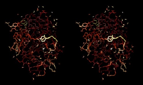
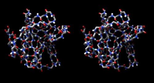
Choose Actions → Atoms/Bonds → stick to give the bonds more volume. You will find that the core of the protein has low temperature factors, and the surface has a number of "glowingly" mobile sidechains and loops.

Structure of the yeast transcription factor Mbp1 DNA binding domain (1BM8) coloured by B-factor (thermal factor). The protein bonds are shown in a "stick" model, coloured with a spectrum that emulates black-body radiation. Note that the interior of the protein is less mobile, some of the surface loops are highly mobile (or statically disordered, X-ray structures can't distinguish that) and the discretely bound water molecules that are visible in this high-resolution structure are generally more mobile than the residues they bind to.

Electrostatics

Task:

To visualize the electrostatic potential of the protein, mapped on the surface, first select Presets → Interactive 2... and Actions → Color → cyan for a vividly contrasting color.
A simple electrostatic potential calculation just assumes Coulomb charges. A more accurate calculation of full Poisson-Boltzmann potentials is also available. Select Tools → Electrostatic/Binding Analysis → Coulombic Surface Coloring.
Make sure the surface object is selected in the form (it should be selected by default since there is only one surface), keep the default parameters and click Apply.
Use Actions → Surface → Transparency → 30% to make the protein backbone somewhat visible.
Open the Tools → Viewing Controls → Lighting window → and set Intensity from two-point to ambient. This reduces shadowing and reflections on the surface and thus emphasizes the color values - here our focus is not on shape, but on property.
Use the Effects tab to turn shadows off and depth-cueing and silhouettes on. This recreates visual cues of depth which compensate for the loss of shape information by using a flat lighting model.

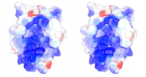
Coulomb (electrostatic) potential mapped to the solvent accessible surface of the yeast transcription factor Mbp1 DNA binding domain (1BM8). The protein backbone is visible through the transparent surface as a cartoon model, note the helix at the bottom of the structure. This helix has been suggested to play a role in forming the domain's DNA binding site and the positive (blue) electrostatic potential of the region is consistent with binding the negatively charged phosphate backbone of DNA. The other side of the domain has a negative (red) charge excess, which balances the molecule's electric charge overall, but also guides the protein-ligand interaction and supports faster on-rates.

Hydrogen bonds

Task:

Hydrogen bonds encode the basic folding patterns of the protein. To visualize H-bonds select Presets → Publication 1... and Actions → Color → by element.
Use Tools → Structure Analysis → FindHBond and Apply default parameters.
To emphasize the role of H-bonds in determining the architecture of the protein, select Select → Structure → backbone → full and then Select → Invert (all models). Now Actions → Atoms/bonds → hide will show only the backbone with its H-bonds.

Hydrogen bonds shown for the peptide backbone of the yeast transcription factor Mbp1 DNA binding domain (1BM8). This view emphasizes the interactions of secondary structure elements that govern the folding topology of the domain.

Chimera sequence interface

In this task we will explore the sequence interface of Chimera, use it to select specific parts of a molecule, and colour specific regions (or residues) of a molecule separately.

Task:

Display the protein in Presets → Interactive 1 mode and familiarize yourself with its topology of helices and strands.
Now turn hydrogen bonds off: the menu commands of Chimera all have a command line equivalent. Open the command line by clicking on the "computer" icon in the upper left corner of the viewer window. Then type "~hbonds". The "~" undoes previous commands.
Use Tools → Depiction → Rainbow to color the chain from blue to red. (You need to change the colour patches by clicking on them to open the colour editor. Choose an HSL colour model, use Saturation and Lightness 0.5 to keep the colour to somewhat subdued hues, then use the slider to choose appropriate hue values.) Click Apply.
Open the sequence tool: Tools → Sequence → Sequence. By default, coloured rectangles overlay the secondary structure elements of the sequence.
Hover the mouse over some residues and note that the sequence number and chain is shown at the bottom of the window.
Click/drag one residue to select it. (Simply a click wont work, you need to drag a little bit for the selection to catch on.) Note that the residue gets a green overlay in the sequence window, and it also gets selected with a green border in the graphics window.
In the bottom of the sequence window, there are instructions how to select (multiple) regions. Clear the selection by <control> clicking into an empty spot of the viewer. Now select the region that encompasses the residues that have been reported to form the DNA binding subdomain: KRTRILEKEVLKETHEKVQGGFGKYQ (Taylor 2000). Show the side chains of these residues by clicking on the little green inspector icon on the viewer window, inspecting Atom and choosing displayed: true, and inspecting Bond and setting the stick radius to 0.4.
Undisplay the Hydrogen atoms by selecting the element H in the Chemistry option of the Selection Menu, and use the Action menu to hide them. Then use the effects pane of the Depiction menu to add a contour.
Finally, give the scene a gradient grey background grey via the Actions → Color → all options... menu.

The DNA binding region of Mbp1 according to NMR measurements of DNA contact by Taylor et al. (2000). The backbone of 1BM8 is shown with a colour ramp from blue (N-terminus) to red (C-terminus). The side chains of the region 50-74 are shown coloured by element.

Chimera "sequence": implicit or explicit ?

You are aware of the distinction between implicit sequence (recorded in the SEQRES records of a PDB file) and explicit sequence (implied by the actual coordinates of the structure). But which of the two does the Chimera sequence window display? Let's find out.

Task:

Open Chimera and load the 1BM8 structure from the PDB.
Save the ccordinate file with File → Save PDB ..., use a filename of test.pdb.
Open this file in a plain text editor: notepad, TextEdit, nano or the like - youcan use RStudio too, but not MS Word! Make sure you view the file in a fixed-width font, not proportionally spaced, i.e. Courier, not Arial. Otherwise the columns in the file won't line up.
Find the records that begin with SEQRES ... and confirm that the first amino acid is GLN.
Now scroll down to the ATOM section of the file. Identify the records for the first residue in the structure. Delete all lines for side-chain atoms except for the CB atom. This changes the coordinates for glutamine to those of alanine.
Replace the GLN residue name with ALA (uppercase). This relabels the residue as Alanine in the coordinate section. Therefore you have changed the implicit sequence. Implicit and explicit sequence are now different. The second atom record should now look like this:

ATOM 2 CA ALA A 4 -0.575 5.127 16.398 1.00 51.22 C

Save the file and load it in Chimera.
Open the sequence window: does it display Q or A as the first reside?

Therefore, does Chimera use the implicit or explicit sequence in the sequence window?

Notes

↑ That's the same effect as when you are watching a 3D movie in the theatre, with polarized glasses: If you have weak posture or a cute neighbour and slouch to the side, your eyes become misaligned relative to the separated images on the screen, your visual system tries to compensate, but over time you get a headache. This is how stereo-haters are bred.

Self-evaluation

If in doubt, ask! If anything about this learning unit is not clear to you, do not proceed blindly but ask for clarification. Post your question on the course mailing list: others are likely to have similar problems. Or send an email to your instructor.

About ...

Author:

Boris Steipe <boris.steipe@utoronto.ca>

Created:

2017-08-05

Modified:

2017-10-17

Version:

1.0

Version history:

1.0 First live version
0.1 First stub - 2016 material combined

This copyrighted material is licensed under a Creative Commons Attribution 4.0 International License. Follow the link to learn more.

[1] That's the same effect as when you are watching a 3D movie in the theatre, with polarized glasses: If you have weak posture or a cute neighbour and slouch to the side, your eyes become misaligned relative to the separated images on the screen, your visual system tries to compensate, but over time you get a headache. This is how stereo-haters are bred.

[1]

BIN-SX-Chimera

Contents

Abstract

This unit ...

Prerequisites

Objectives

Outcomes

Deliverables

Evaluation

Contents

Molecular graphics: UCSF Chimera

Chimera: First steps

Stereo Viewing

Physiology

Practice

Global properties

A Ramachandran plot

B-factors

Electrostatics

Hydrogen bonds

Chimera sequence interface

Chimera "sequence": implicit or explicit ?

Further reading, links and resources

Notes

Self-evaluation

Navigation menu

Personal tools

Namespaces

Variants

Views

More

Search

Sections

Tools