Difference between revisions of "Lecture 05"
Jump to navigation
Jump to search


| (6 intermediate revisions by the same user not shown) | |||
| Line 1: | Line 1: | ||
| + | <!-- div style="padding: 5px; background: #FF4560; border:solid 2px #000000;"> | ||
| + | '''Update Warning!''' | ||
| + | This page has not been revised yet for the 2007 Fall term. Some of the slides may be reused, but please consider the page as a whole out of date as long as this warning appears here. | ||
| + | </div --> | ||
| + | | ||
| + | |||
| + | | ||
| + | |||
__NOTOC__ | __NOTOC__ | ||
<small>[[Lecture_04|(Previous lecture)]] ... [[Lecture_06|(Next lecture)]]</small> | <small>[[Lecture_04|(Previous lecture)]] ... [[Lecture_06|(Next lecture)]]</small> | ||
| + | <div style="padding: 5px; background: #A6AFD0; border:solid 1px #AAAAAA; font-size:150%;font-weight:bold;"> | ||
==Homology - I: the Principles== | ==Homology - I: the Principles== | ||
| + | </div> | ||
| + | |||
| + | ;What you should take home from this part of the course: | ||
| + | |||
| + | *Understand what homology means and what can be deduced from the fact that two sequences are homologues. | ||
| + | *Understand that the similarity of amino acids' biological functions depends on the amino acid but also on the context. | ||
| + | *Know that sequence similarity can be measured, based on amino acid pair scores. | ||
| + | *Be familiar with the concept of a scoring matrix and with scoring matrices in common use for sequence alignment; appreciate the differences between these matrices and the '''models''' embodied in them. | ||
| + | *Be familiar with the principle of a dotplot and tools to generate a dotplot. | ||
| + | | ||
| + | |||
| + | |||
| + | ;Links summary: | ||
| + | *The [http://www.isrec.isb-sib.ch/java/dotlet/Dotlet.html '''Dotlet''' applet] on the Web. | ||
| + | | ||
| − | ... | + | ;Exercises |
| + | *Read [http://biochemistry.utoronto.ca/undergraduates/courses/BCH441H/restricted/Fitch_HomologyDefinitions.pdf '''Walter Fitch's review''' (pdf)] (2000, ''Trends Genet'' '''16''':227-231) on the topic of homology and familiarize yourself with the concepts! | ||
| + | *Read [http://www.nature.com/nbt/journal/v22/n8/full/nbt0804-1035.html '''Sean Eddy's summary'''] (2004, ''Nat Biotechnol.'' '''8''':1035-1036) of the theory behind and the development of the BLOSUM62 matrix. | ||
| + | | ||
| + | | ||
| − | + | <div style="padding: 5px; background: #A6AFD0; border:solid 1px #AAAAAA; font-size:150%;font-weight:bold;"> | |
| − | |||
| − | |||
| − | |||
==Lecture Slides== | ==Lecture Slides== | ||
| + | </div> | ||
======Slide 001====== | ======Slide 001====== | ||
[[Image:L05_s001.jpg|frame|none|Lecture 05, Slide 001<br> | [[Image:L05_s001.jpg|frame|none|Lecture 05, Slide 001<br> | ||
| + | It is commonplace today that far-reaching conclusions about biological function are drawn from the inference of homology between proteins or protein domains. | ||
| + | ]] | ||
| + | |||
| + | <div style="padding: 2px; background: #F0F1F7; border:solid 1px #AAAAAA; font-size:125%;color:#444444"> | ||
| + | ===The concept of homology=== | ||
| + | </div> | ||
| − | |||
======Slide 002====== | ======Slide 002====== | ||
[[Image:L05_s002.jpg|frame|none|Lecture 05, Slide 002<br> | [[Image:L05_s002.jpg|frame|none|Lecture 05, Slide 002<br> | ||
| − | + | The concept of homologous sequences is extensively applied wherever genes or organisms are compared. It is especially important for the study of biology through ''Model organisms'', where inferences about one species are made from data gathered in another. These inferences are justified, because (and to the degree that) the species are related ... | |
]] | ]] | ||
======Slide 003====== | ======Slide 003====== | ||
[[Image:L05_s003.jpg|frame|none|Lecture 05, Slide 003<br> | [[Image:L05_s003.jpg|frame|none|Lecture 05, Slide 003<br> | ||
| − | + | The word '''Homology''' has a precise meaning (in biology) and should not be used differently! Read [http://biochemistry.utoronto.ca/undergraduates/courses/BCH441H/restricted/Fitch_HomologyDefinitions.pdf '''Walter Fitch's excellent review'''] (2000, ''Trends Genet'' '''16''':227-231) on the topic.<br> <br>We conjecture that paralogous genes have similar but importantly different functions because otherwise one of the copies would be superfluous ,and would be lost under evolutionary drift. Note that we are especially interested in orthologous relationships, because we infer that two orthologues would have maintained the "same" functions. However please note that when one or both organisms have undergone additional duplications after speciation, multiple orthologues may exist. Fitch has proposed the term '''isoorthologues''' for that pair of genes with the "same" function among a family. While this is an excellent proposal that would address much confusion, unfortunately the term has not caught on. Thus, rather than rely on a shared understanding of expansive vocabulary in the community, define your concepts explicitly and adhere to your definitions. | |
]] | ]] | ||
======Slide 004====== | ======Slide 004====== | ||
| Line 32: | Line 63: | ||
======Slide 005====== | ======Slide 005====== | ||
[[Image:L05_s005.jpg|frame|none|Lecture 05, Slide 005<br> | [[Image:L05_s005.jpg|frame|none|Lecture 05, Slide 005<br> | ||
| − | + | The equivalence principle might not be obvious. Given that the cenancestral sequences (the last common ancestor sequences) of the pairs {A,B} and {B,C} are different, how do those relationships tell us something about the relationship between {A,C}? | |
]] | ]] | ||
======Slide 006====== | ======Slide 006====== | ||
[[Image:L05_s006.jpg|frame|none|Lecture 05, Slide 006<br> | [[Image:L05_s006.jpg|frame|none|Lecture 05, Slide 006<br> | ||
| − | + | The answer is based on the fact that there are two, but only two, possibilities for the relationship between {A,B} and {B,C}, drawn above <small>(assuming a simple, dichotomous branching relation between the genes)</small>. (1): the divergence between {B,C} happened '''before''' {A,B}, at node ''y''. (2): the divergence between {B,C} happened '''after''' {A,B}, at node ''z''. Thus we do not know '''which''' of the cases is the correct one, the ancestral gene for all three genes can be either ''x'' or ''y'' ... | |
]] | ]] | ||
======Slide 007====== | ======Slide 007====== | ||
[[Image:L05_s007.jpg|frame|none|Lecture 05, Slide 007<br> | [[Image:L05_s007.jpg|frame|none|Lecture 05, Slide 007<br> | ||
| − | + | ... but we do know that '''some common ancestral gene exists''' for all three sequences, and therefore they must all three be homologous. | |
]] | ]] | ||
======Slide 008====== | ======Slide 008====== | ||
| Line 54: | Line 85: | ||
]] | ]] | ||
| + | |||
| + | <div style="padding: 2px; background: #F0F1F7; border:solid 1px #AAAAAA; font-size:125%;color:#444444"> | ||
| + | ===Inferring homology=== | ||
| + | </div> | ||
| + | |||
======Slide 011====== | ======Slide 011====== | ||
[[Image:L05_s011.jpg|frame|none|Lecture 05, Slide 011<br> | [[Image:L05_s011.jpg|frame|none|Lecture 05, Slide 011<br> | ||
| − | + | Many obviously homologous genes have very low sequence identity. In this example, the aligned sequences of green- and red- fluorescent protein share 57 of 239 identical residues, i.e. the sequence identity is 23.8%. | |
]] | ]] | ||
======Slide 012====== | ======Slide 012====== | ||
[[Image:L05_s012.jpg|frame|none|Lecture 05, Slide 012<br> | [[Image:L05_s012.jpg|frame|none|Lecture 05, Slide 012<br> | ||
| − | + | Obviously, the fraction of identical residues depends on the alignment and we need to consider how the right alignment can be obtained. But even before we can start aligning, we need to define a metric between amino acids, to quantify amino acid similarity because the right alignment should give us good '''similarity''', not just a large percentage of '''identical''' residues. So the second issue comes before the first issue. And there is an additional second issue: how do we treat sequence insertions resp. deletions in the alignment? | |
]] | ]] | ||
======Slide 013====== | ======Slide 013====== | ||
| Line 66: | Line 102: | ||
]] | ]] | ||
| + | |||
| + | <div style="padding: 2px; background: #F0F1F7; border:solid 1px #AAAAAA; font-size:125%;color:#444444"> | ||
| + | ===Measuring amino acid similarity=== | ||
| + | </div> | ||
| + | |||
======Slide 014====== | ======Slide 014====== | ||
[[Image:L05_s014.jpg|frame|none|Lecture 05, Slide 014<br> | [[Image:L05_s014.jpg|frame|none|Lecture 05, Slide 014<br> | ||
| + | Biophysical amino acid properties can be used to group amino acids into sets. Each memebr of this set could be considered to be similar, according to that property. Alternatively, biophysical properties can be tabulated and similarity computed according to a scale. Such numerical scales may include properties as | ||
| + | *the free energy of transfer from water to octanol;<br> | ||
| + | *the pKa of the sidechain;<br> | ||
| + | *the volume;<br> | ||
| + | *the accessible surface area (ASA), and many more.<br> | ||
| + | <br> | ||
| + | For more details, see the [http://en.wikipedia.org/wiki/List_of_standard_amino_acids Wikipedia article] on the standard amino acids. | ||
]] | ]] | ||
======Slide 015====== | ======Slide 015====== | ||
[[Image:L05_s015.jpg|frame|none|Lecture 05, Slide 015<br> | [[Image:L05_s015.jpg|frame|none|Lecture 05, Slide 015<br> | ||
| − | + | In a sequence, all information about the molecular properties of an amino acid is condensed into into the single letter code (or other labels for "abstractions" of amino acids). However, how similar one amino acid is to other amino acids depends on the role it plays for the structure and/or function of a protein. Depending on this role, an amino acid like tyrosine would be considered e.g. similar to other ''hydrophobic'' amino acids, or other side chains that can accept H-bonds. However these two groups are non-overlapping sets! | |
]] | ]] | ||
======Slide 016====== | ======Slide 016====== | ||
| Line 82: | Line 130: | ||
]] | ]] | ||
| + | |||
| + | <div style="padding: 2px; background: #F0F1F7; border:solid 1px #AAAAAA; font-size:125%;color:#444444"> | ||
| + | ===Scoring matrices=== | ||
| + | </div> | ||
| + | |||
| + | |||
======Slide 018====== | ======Slide 018====== | ||
[[Image:L05_s018.jpg|frame|none|Lecture 05, Slide 018<br> | [[Image:L05_s018.jpg|frame|none|Lecture 05, Slide 018<br> | ||
| − | + | A scoring matrix is a computational tool that associates each pair of residues with a number. In this example, the score of the pair {E,D} from an alignment is read out from a scoring matrix. | |
]] | ]] | ||
======Slide 019====== | ======Slide 019====== | ||
[[Image:L05_s019.jpg|frame|none|Lecture 05, Slide 019<br> | [[Image:L05_s019.jpg|frame|none|Lecture 05, Slide 019<br> | ||
| − | + | The Identity Matrix is valid only at small evolutionary distances (where all similarity matrices give comparable results). Currently, it is primarily used for nucleotide sequence comparisons, where the concept of ''similarity'' does not really apply. But the more realistic the model of the evolutionary process is, the less information is discarded. Better models make less assumptions. Many interesting biological relationships have been uncovered precisely because we have been able to perform very sensitive homology searches. | |
]] | ]] | ||
======Slide 020====== | ======Slide 020====== | ||
[[Image:L05_s020.jpg|frame|none|Lecture 05, Slide 020<br> | [[Image:L05_s020.jpg|frame|none|Lecture 05, Slide 020<br> | ||
| − | + | There is more to this matrix than might seem apparent. Mechanistically speaking, similar codons arise from single nucleotide changes. But functionally speaking, the genetic code [http://www.ncbi.nlm.nih.gov/sites/entrez?Db=pubmed&Cmd=ShowDetailView&TermToSearch=9732450 minimizes the biophysical effect of mutations]! Thus similar codons code for "similar" amino acids. | |
]] | ]] | ||
======Slide 021====== | ======Slide 021====== | ||
[[Image:L05_s021.jpg|frame|none|Lecture 05, Slide 021<br> | [[Image:L05_s021.jpg|frame|none|Lecture 05, Slide 021<br> | ||
| − | + | The model that M.O. Dayhoff proposed in 1978 departs from an ''ab initio'' attempt to define amino acid similarity to an empirical approach. | |
]] | ]] | ||
======Slide 022====== | ======Slide 022====== | ||
| Line 104: | Line 158: | ||
======Slide 023====== | ======Slide 023====== | ||
[[Image:L05_s023.jpg|frame|none|Lecture 05, Slide 023<br> | [[Image:L05_s023.jpg|frame|none|Lecture 05, Slide 023<br> | ||
| − | + | The matrix above is not the Dayhoff matrix, it is just called "MDM". It was derived from the original 1978 Dayhoff matrix for PAM250 by rescaling it to give a constant score for identities (1.5). This may save computational resources but is an unfounded, arbitrary change. Nevertheless, this matrix was the one that was in most common use for many years. | |
]] | ]] | ||
======Slide 024====== | ======Slide 024====== | ||
[[Image:L05_s024.jpg|frame|none|Lecture 05, Slide 024<br> | [[Image:L05_s024.jpg|frame|none|Lecture 05, Slide 024<br> | ||
| − | + | Two of arginine's six codons (CGG and AGG) can be changed to the tryptophan codon TGG by a single point mutation. Thus these two amino acids, which have quite different biophysical properties and distributions, are defined as almost as ''similar'' as a pair of identitcal amino acids by this matrix that was constructed by extrapolation from highly related sequences. The source data that M.O. Dayhoff had used was biased towards sequences in which secondary, functional selection may not have had time to occur after an initial mutation event. Accordingly, this process of extrapolation is expected to inappropriately favour exchanges that can be coded by a single nucleotide substitution. Thus, while the model is rigorous and well designed, the source data limits its accuracy.<br> | |
| + | <br> | ||
| + | The inset picture shows the relationship between '''PAM''' - percent accepted mutation and % residue identity. This is '''not''' a linear relationship, due to back-mutation. In the limit of infinitely many accepted mutations, sequence identity should still be around 5% and not 0. | ||
]] | ]] | ||
======Slide 025====== | ======Slide 025====== | ||
| Line 116: | Line 172: | ||
======Slide 026====== | ======Slide 026====== | ||
[[Image:L05_s026.jpg|frame|none|Lecture 05, Slide 026<br> | [[Image:L05_s026.jpg|frame|none|Lecture 05, Slide 026<br> | ||
| − | + | Read [http://www.nature.com/nbt/journal/v22/n8/full/nbt0804-1035.html Sean Eddy's excellent summary] of the theory behind and the development of the BLOSUM62 matrix. | |
]] | ]] | ||
======Slide 027====== | ======Slide 027====== | ||
| Line 123: | Line 179: | ||
]] | ]] | ||
======Slide 028====== | ======Slide 028====== | ||
| − | + | (deleted) | |
| + | |||
| + | |||
| + | <div style="padding: 2px; background: #F0F1F7; border:solid 1px #AAAAAA; font-size:125%;color:#444444"> | ||
| + | ===Sequence comparison: Dotplots=== | ||
| + | </div> | ||
| + | |||
| − | |||
======Slide 029====== | ======Slide 029====== | ||
[[Image:L05_s029.jpg|frame|none|Lecture 05, Slide 029<br> | [[Image:L05_s029.jpg|frame|none|Lecture 05, Slide 029<br> | ||
| − | + | For examples of biological sequence features in a dotplot: see [<b>http://www.isrec.isb-sib.ch/java/dotlet/dotlet_examples.html '''here'''].</b> | |
]] | ]] | ||
======Slide 030====== | ======Slide 030====== | ||
[[Image:L05_s030.jpg|frame|none|Lecture 05, Slide 030<br> | [[Image:L05_s030.jpg|frame|none|Lecture 05, Slide 030<br> | ||
| − | + | The [<b>http://www.isrec.isb-sib.ch/java/dotlet/Dotlet.html </b>'''Dotlet''' applet] on the Web. A of standalone tool for local installation is [http://www.cgr.ki.se/cgr/groups/sonnhammer/Dotter.html '''Dotter'''], also available on the Web as [http://athena.bioc.uvic.ca/workbench.php?tool=jdotter JDotter]. | |
]] | ]] | ||
| − | |||
| − | |||
| − | + | | |
| − | + | | |
| − | [[ | + | ---- |
| − | + | <small>[[Lecture_04|(Previous lecture)]] ... [[Lecture_06|(Next lecture)]]</small> | |
| − | |||
Latest revision as of 12:53, 25 September 2007
(Previous lecture) ... (Next lecture)
Homology - I: the Principles
- What you should take home from this part of the course
- Understand what homology means and what can be deduced from the fact that two sequences are homologues.
- Understand that the similarity of amino acids' biological functions depends on the amino acid but also on the context.
- Know that sequence similarity can be measured, based on amino acid pair scores.
- Be familiar with the concept of a scoring matrix and with scoring matrices in common use for sequence alignment; appreciate the differences between these matrices and the models embodied in them.
- Be familiar with the principle of a dotplot and tools to generate a dotplot.
- Links summary
- The Dotlet applet on the Web.
- Exercises
- Read Walter Fitch's review (pdf) (2000, Trends Genet 16:227-231) on the topic of homology and familiarize yourself with the concepts!
- Read Sean Eddy's summary (2004, Nat Biotechnol. 8:1035-1036) of the theory behind and the development of the BLOSUM62 matrix.
Lecture Slides
Slide 001

Lecture 05, Slide 001
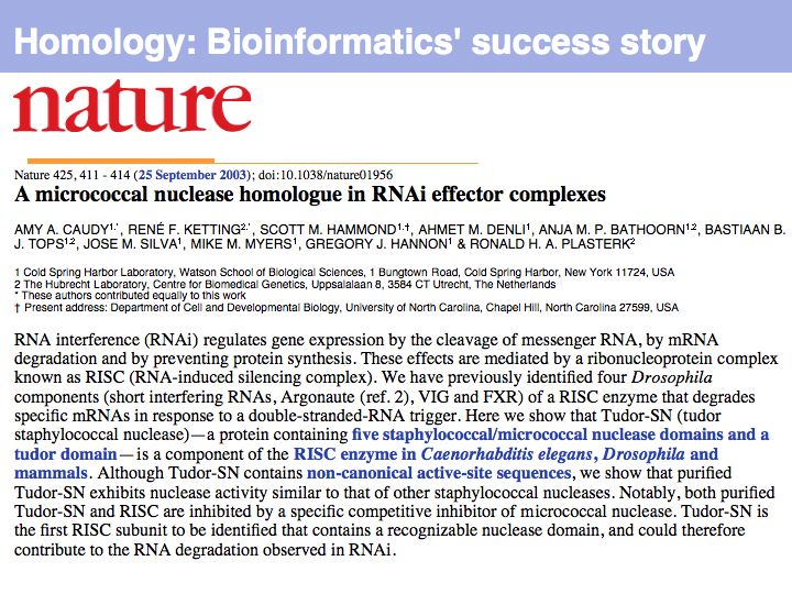
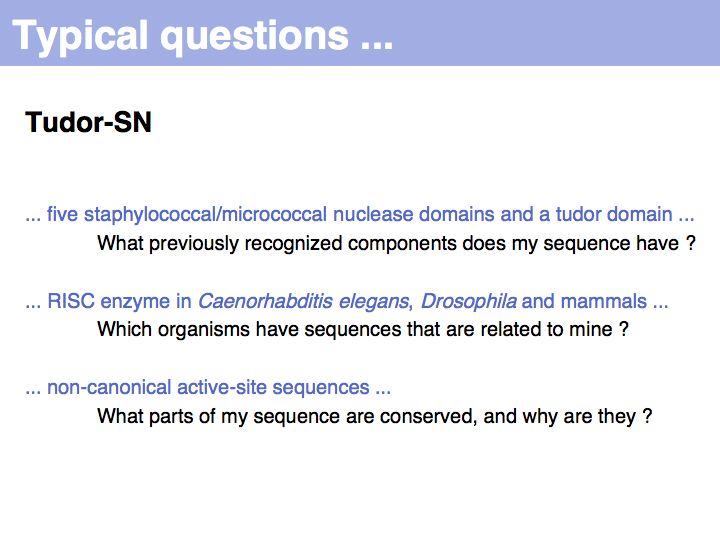
It is commonplace today that far-reaching conclusions about biological function are drawn from the inference of homology between proteins or protein domains.
It is commonplace today that far-reaching conclusions about biological function are drawn from the inference of homology between proteins or protein domains.
The concept of homology
Slide 002

Lecture 05, Slide 002
The concept of homologous sequences is extensively applied wherever genes or organisms are compared. It is especially important for the study of biology through Model organisms, where inferences about one species are made from data gathered in another. These inferences are justified, because (and to the degree that) the species are related ...
The concept of homologous sequences is extensively applied wherever genes or organisms are compared. It is especially important for the study of biology through Model organisms, where inferences about one species are made from data gathered in another. These inferences are justified, because (and to the degree that) the species are related ...
Slide 003

Lecture 05, Slide 003
The word Homology has a precise meaning (in biology) and should not be used differently! Read Walter Fitch's excellent review (2000, Trends Genet 16:227-231) on the topic.
We conjecture that paralogous genes have similar but importantly different functions because otherwise one of the copies would be superfluous ,and would be lost under evolutionary drift. Note that we are especially interested in orthologous relationships, because we infer that two orthologues would have maintained the "same" functions. However please note that when one or both organisms have undergone additional duplications after speciation, multiple orthologues may exist. Fitch has proposed the term isoorthologues for that pair of genes with the "same" function among a family. While this is an excellent proposal that would address much confusion, unfortunately the term has not caught on. Thus, rather than rely on a shared understanding of expansive vocabulary in the community, define your concepts explicitly and adhere to your definitions.
Slide 004

Lecture 05, Slide 004
Slide 005

Lecture 05, Slide 005
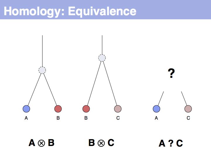
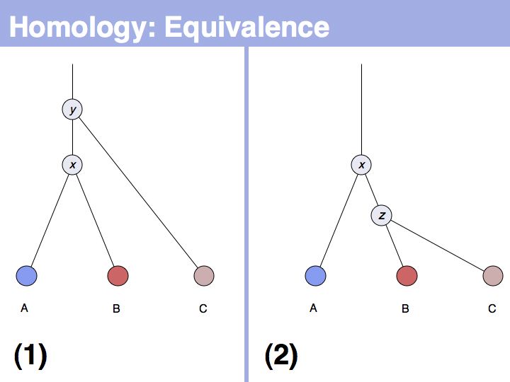
The equivalence principle might not be obvious. Given that the cenancestral sequences (the last common ancestor sequences) of the pairs {A,B} and {B,C} are different, how do those relationships tell us something about the relationship between {A,C}?
The equivalence principle might not be obvious. Given that the cenancestral sequences (the last common ancestor sequences) of the pairs {A,B} and {B,C} are different, how do those relationships tell us something about the relationship between {A,C}?
Slide 006

Lecture 05, Slide 006
The answer is based on the fact that there are two, but only two, possibilities for the relationship between {A,B} and {B,C}, drawn above (assuming a simple, dichotomous branching relation between the genes). (1): the divergence between {B,C} happened before {A,B}, at node y. (2): the divergence between {B,C} happened after {A,B}, at node z. Thus we do not know which of the cases is the correct one, the ancestral gene for all three genes can be either x or y ...
The answer is based on the fact that there are two, but only two, possibilities for the relationship between {A,B} and {B,C}, drawn above (assuming a simple, dichotomous branching relation between the genes). (1): the divergence between {B,C} happened before {A,B}, at node y. (2): the divergence between {B,C} happened after {A,B}, at node z. Thus we do not know which of the cases is the correct one, the ancestral gene for all three genes can be either x or y ...
Slide 007

Lecture 05, Slide 007
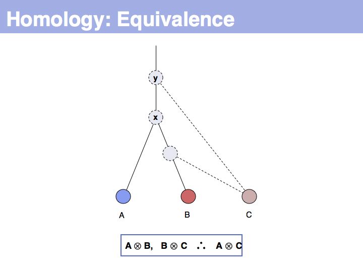
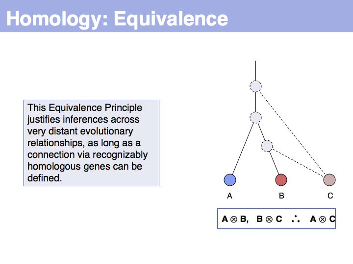
... but we do know that some common ancestral gene exists for all three sequences, and therefore they must all three be homologous.
... but we do know that some common ancestral gene exists for all three sequences, and therefore they must all three be homologous.
Slide 008

Lecture 05, Slide 008
Slide 009

Lecture 05, Slide 009
Slide 010

Lecture 05, Slide 010
Inferring homology
Slide 011

Lecture 05, Slide 011
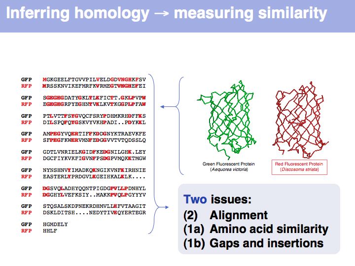
Many obviously homologous genes have very low sequence identity. In this example, the aligned sequences of green- and red- fluorescent protein share 57 of 239 identical residues, i.e. the sequence identity is 23.8%.
Many obviously homologous genes have very low sequence identity. In this example, the aligned sequences of green- and red- fluorescent protein share 57 of 239 identical residues, i.e. the sequence identity is 23.8%.
Slide 012

Lecture 05, Slide 012
Obviously, the fraction of identical residues depends on the alignment and we need to consider how the right alignment can be obtained. But even before we can start aligning, we need to define a metric between amino acids, to quantify amino acid similarity because the right alignment should give us good similarity, not just a large percentage of identical residues. So the second issue comes before the first issue. And there is an additional second issue: how do we treat sequence insertions resp. deletions in the alignment?
Obviously, the fraction of identical residues depends on the alignment and we need to consider how the right alignment can be obtained. But even before we can start aligning, we need to define a metric between amino acids, to quantify amino acid similarity because the right alignment should give us good similarity, not just a large percentage of identical residues. So the second issue comes before the first issue. And there is an additional second issue: how do we treat sequence insertions resp. deletions in the alignment?
Slide 013

Lecture 05, Slide 013
Measuring amino acid similarity
Slide 014

Lecture 05, Slide 014
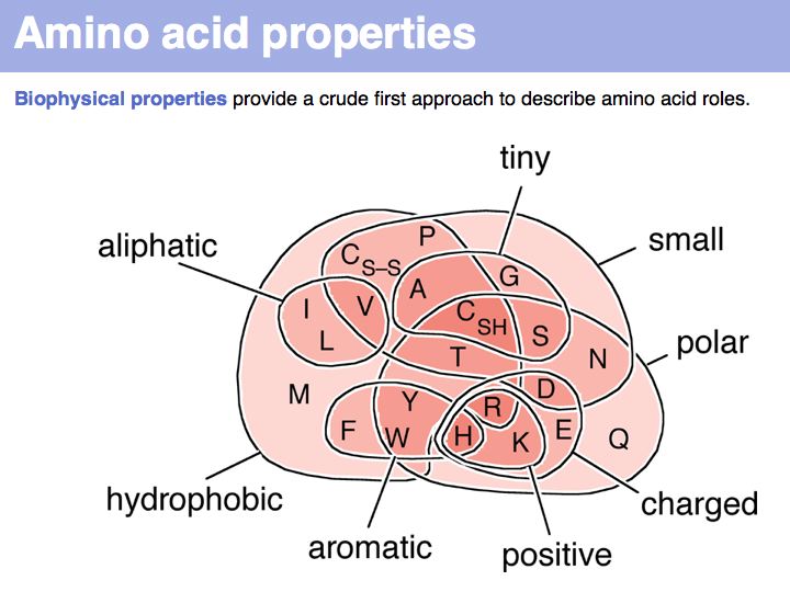
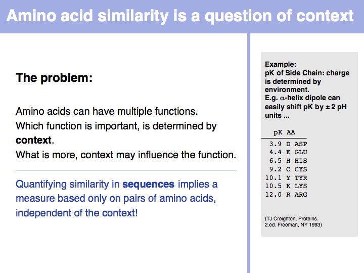
Biophysical amino acid properties can be used to group amino acids into sets. Each memebr of this set could be considered to be similar, according to that property. Alternatively, biophysical properties can be tabulated and similarity computed according to a scale. Such numerical scales may include properties as *the free energy of transfer from water to octanol;
*the pKa of the sidechain;
*the volume;
*the accessible surface area (ASA), and many more.
For more details, see the Wikipedia article on the standard amino acids.
Slide 015

Lecture 05, Slide 015
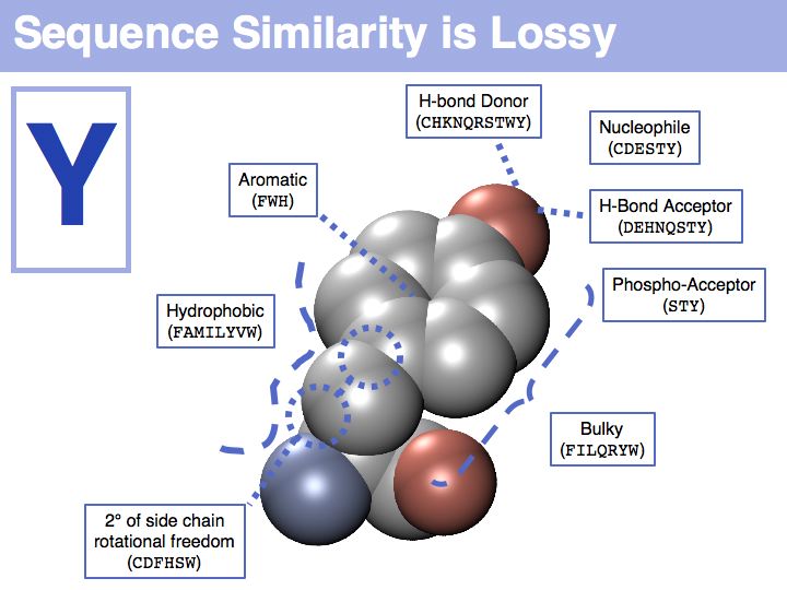
In a sequence, all information about the molecular properties of an amino acid is condensed into into the single letter code (or other labels for "abstractions" of amino acids). However, how similar one amino acid is to other amino acids depends on the role it plays for the structure and/or function of a protein. Depending on this role, an amino acid like tyrosine would be considered e.g. similar to other hydrophobic amino acids, or other side chains that can accept H-bonds. However these two groups are non-overlapping sets!
In a sequence, all information about the molecular properties of an amino acid is condensed into into the single letter code (or other labels for "abstractions" of amino acids). However, how similar one amino acid is to other amino acids depends on the role it plays for the structure and/or function of a protein. Depending on this role, an amino acid like tyrosine would be considered e.g. similar to other hydrophobic amino acids, or other side chains that can accept H-bonds. However these two groups are non-overlapping sets!
Slide 016

Lecture 05, Slide 016
Slide 017

Lecture 05, Slide 017
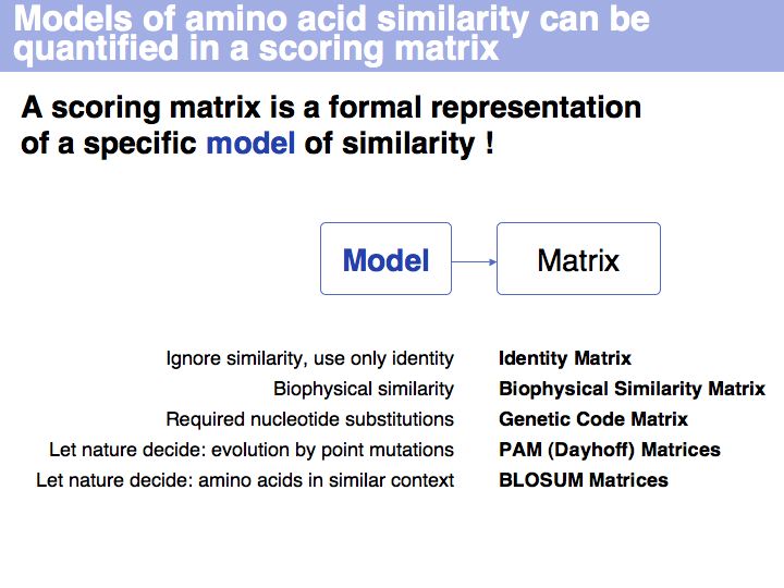
Scoring matrices
Slide 018

Lecture 05, Slide 018
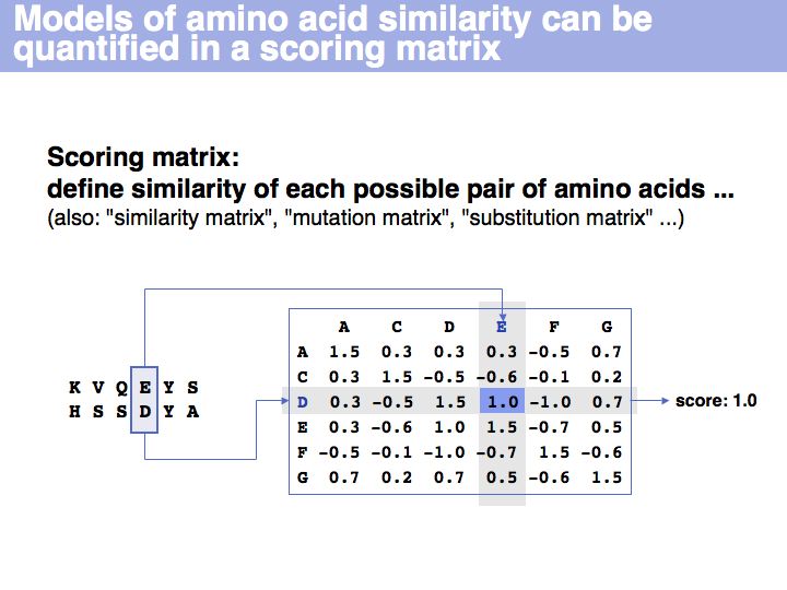
A scoring matrix is a computational tool that associates each pair of residues with a number. In this example, the score of the pair {E,D} from an alignment is read out from a scoring matrix.
A scoring matrix is a computational tool that associates each pair of residues with a number. In this example, the score of the pair {E,D} from an alignment is read out from a scoring matrix.
Slide 019

Lecture 05, Slide 019
The Identity Matrix is valid only at small evolutionary distances (where all similarity matrices give comparable results). Currently, it is primarily used for nucleotide sequence comparisons, where the concept of similarity does not really apply. But the more realistic the model of the evolutionary process is, the less information is discarded. Better models make less assumptions. Many interesting biological relationships have been uncovered precisely because we have been able to perform very sensitive homology searches.
The Identity Matrix is valid only at small evolutionary distances (where all similarity matrices give comparable results). Currently, it is primarily used for nucleotide sequence comparisons, where the concept of similarity does not really apply. But the more realistic the model of the evolutionary process is, the less information is discarded. Better models make less assumptions. Many interesting biological relationships have been uncovered precisely because we have been able to perform very sensitive homology searches.
Slide 020

Lecture 05, Slide 020
There is more to this matrix than might seem apparent. Mechanistically speaking, similar codons arise from single nucleotide changes. But functionally speaking, the genetic code minimizes the biophysical effect of mutations! Thus similar codons code for "similar" amino acids.
There is more to this matrix than might seem apparent. Mechanistically speaking, similar codons arise from single nucleotide changes. But functionally speaking, the genetic code minimizes the biophysical effect of mutations! Thus similar codons code for "similar" amino acids.
Slide 021

Lecture 05, Slide 021
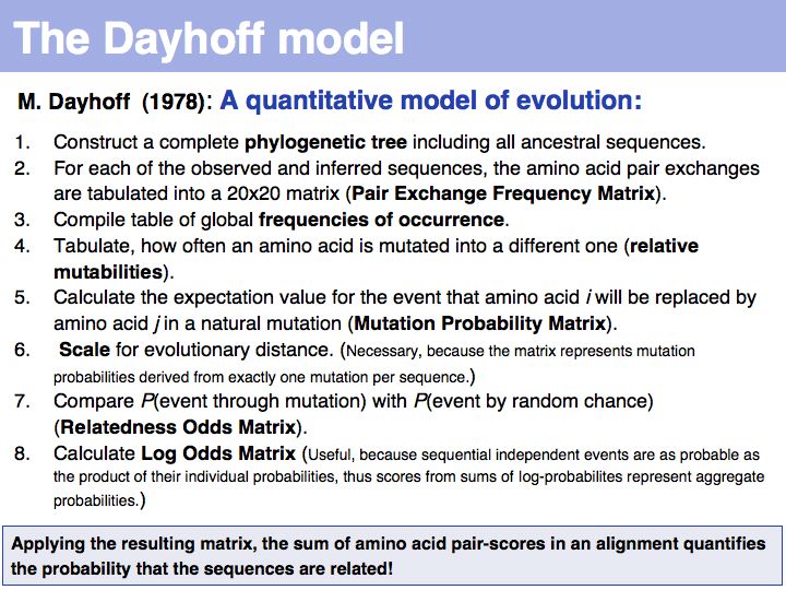
The model that M.O. Dayhoff proposed in 1978 departs from an ab initio attempt to define amino acid similarity to an empirical approach.
The model that M.O. Dayhoff proposed in 1978 departs from an ab initio attempt to define amino acid similarity to an empirical approach.
Slide 022

Lecture 05, Slide 022
Slide 023

Lecture 05, Slide 023
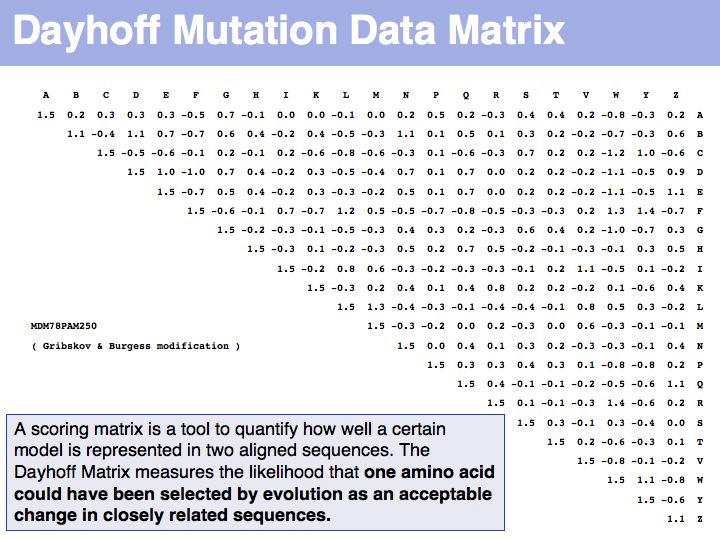
The matrix above is not the Dayhoff matrix, it is just called "MDM". It was derived from the original 1978 Dayhoff matrix for PAM250 by rescaling it to give a constant score for identities (1.5). This may save computational resources but is an unfounded, arbitrary change. Nevertheless, this matrix was the one that was in most common use for many years.
The matrix above is not the Dayhoff matrix, it is just called "MDM". It was derived from the original 1978 Dayhoff matrix for PAM250 by rescaling it to give a constant score for identities (1.5). This may save computational resources but is an unfounded, arbitrary change. Nevertheless, this matrix was the one that was in most common use for many years.
Slide 024

Lecture 05, Slide 024
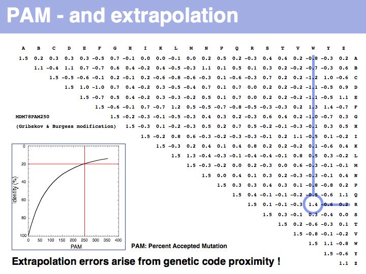
Two of arginine's six codons (CGG and AGG) can be changed to the tryptophan codon TGG by a single point mutation. Thus these two amino acids, which have quite different biophysical properties and distributions, are defined as almost as similar as a pair of identitcal amino acids by this matrix that was constructed by extrapolation from highly related sequences. The source data that M.O. Dayhoff had used was biased towards sequences in which secondary, functional selection may not have had time to occur after an initial mutation event. Accordingly, this process of extrapolation is expected to inappropriately favour exchanges that can be coded by a single nucleotide substitution. Thus, while the model is rigorous and well designed, the source data limits its accuracy.
The inset picture shows the relationship between PAM - percent accepted mutation and % residue identity. This is not a linear relationship, due to back-mutation. In the limit of infinitely many accepted mutations, sequence identity should still be around 5% and not 0.
Slide 025

Lecture 05, Slide 025
Slide 026

Lecture 05, Slide 026
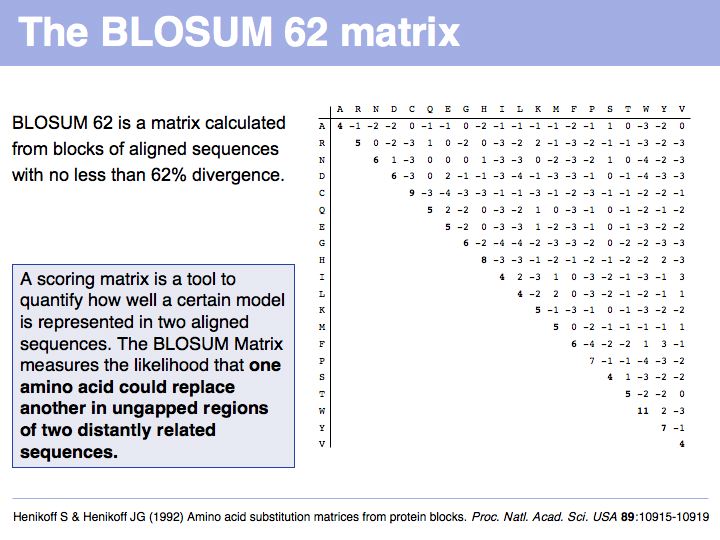
Read Sean Eddy's excellent summary of the theory behind and the development of the BLOSUM62 matrix.
Read Sean Eddy's excellent summary of the theory behind and the development of the BLOSUM62 matrix.
Slide 027

Lecture 05, Slide 027
Slide 028
(deleted)
Sequence comparison: Dotplots
Slide 029

Lecture 05, Slide 029
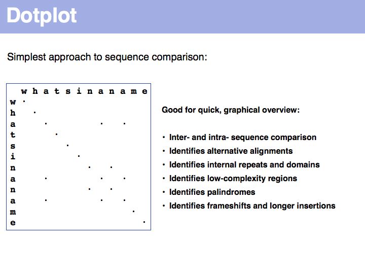
For examples of biological sequence features in a dotplot: see [http://www.isrec.isb-sib.ch/java/dotlet/dotlet_examples.html here].
For examples of biological sequence features in a dotplot: see [http://www.isrec.isb-sib.ch/java/dotlet/dotlet_examples.html here].
Slide 030

Lecture 05, Slide 030
The [http://www.isrec.isb-sib.ch/java/dotlet/Dotlet.html Dotlet applet] on the Web. A of standalone tool for local installation is Dotter, also available on the Web as JDotter.
The [http://www.isrec.isb-sib.ch/java/dotlet/Dotlet.html Dotlet applet] on the Web. A of standalone tool for local installation is Dotter, also available on the Web as JDotter.