Lecture 06
Jump to navigation
Jump to search
(Previous lecture) ... (Next lecture)
Homology II: Optimal Sequence Alignment
Objectives for this part of the course
- Understand that homology is inferred from optimal sequence alignments, by using scoring matrices that represent an evolutionary relationship.
- Understand the principle of how a dynamic programming alignment works by optimizing the sum of pairscores, using an affine gap model for indels, and backtracking to reconstruct an alignment from contributing cells.
- Have a sense for problems associated with affine gap functions and how parameter choice influences size and distribution of indels.
- Understand the difference between global and local optimal alignment and in which situation these algorithms are appropriately used.
- Confidently determine which input sequence to use for an alignment and how to set parameters.
- Be familiar with key Web tools for optimal sequence alignment and detection of repeats.
- Be able to interpret an alignment score and know about empirical thresholds for "homology".
Links summary
- "Recursion" - read here
- Memoization
- Shuffle-LAGAN
- Needleman-Wunsch algorithm for global, optimal sequence alignment
- Dynamic Programming
- larger, explicit example
- Qian and Goldstein (2001)
- Cartwright, 2006
- CDART database
- RADAR server
- Mbp1
- Swi4
- EMBOSS GUI
Exercises
- Retrieve the sequences for Mbp1 and Swi4 from NCBI and access one of the EMBOSS GUI servers.
- Perform a global optimal sequence alignment with the program needle. Note the regions of poor alignment. Note the global alignment score and % identity. Change the parameters for gap opening and gap extension and see what influence this has on the alignment.Then change the scoring matrix to a matrix suitable for very similar sequences, to one that is suitable for highly diverged sequences.
- Perfom a local optimal sequence alignment with the program water. You should likely only get a much shorter, conserved domain - the DNA binding "APSES" domain aligned. Do you think you are missing homologous sequence here?
- Delete the APSES domains from the input sequence and rerun the local alignment. Do you get other, conserved domains aligned?
- Finally, compare the results of your local alignment and the global alignment. Are there differences?
Lecture slides
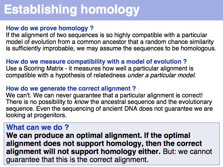
Homology and optimal alignment
Slide 005

Lecture 06, Slide 005
Slide 006

Lecture 06, Slide 006
Slide 007

Lecture 06, Slide 007
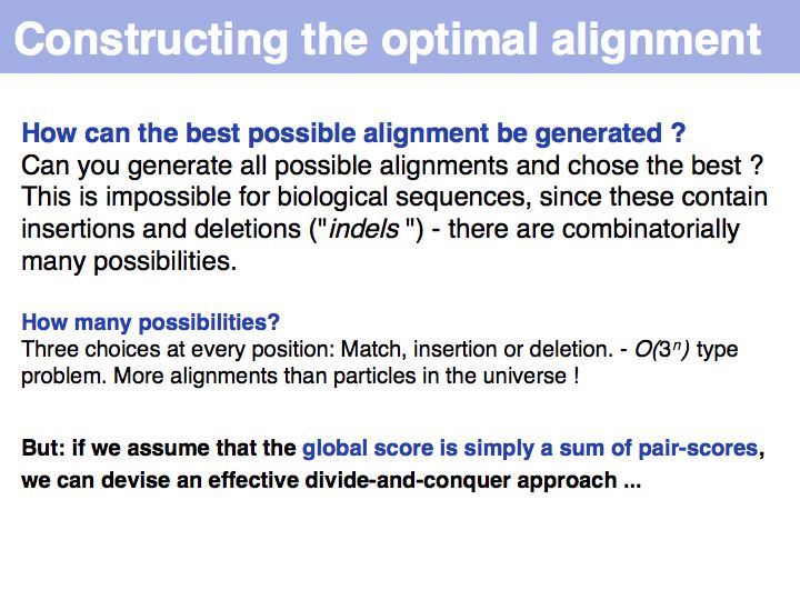
Number of particles in the universe: on the order of 1081. Alignments for two sequences of length 200: ~3200 = 1095.
Number of particles in the universe: on the order of 1081. Alignments for two sequences of length 200: ~3200 = 1095.
Slide 008

Lecture 06, Slide 008
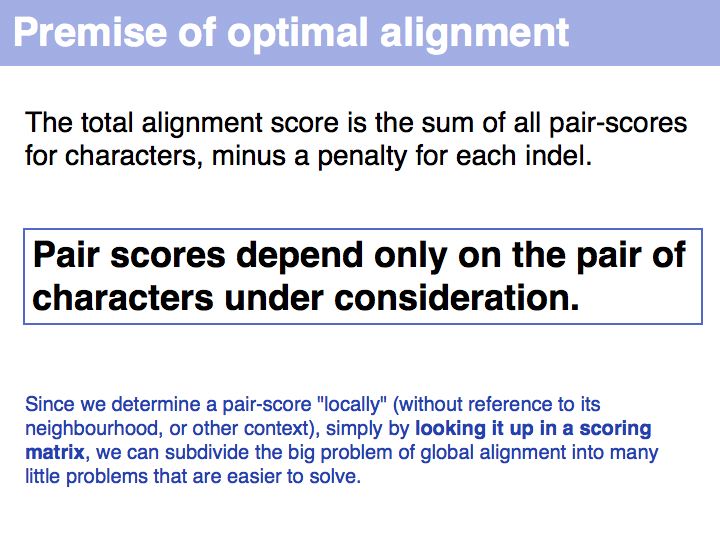
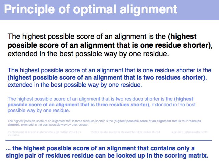
The premise of context independence makes finding an optimal alignment a solvable problem. It is can be shown that alignment problems that are not context-independent are NP hard, i.e. no algorithm exists that solves such a problem in a number of steps that is proportional to some polynomial of the alignment length. Rather, the number of steps in fully context-sensitive, gapped alignment must be proportional to some number to the power of the alignment length. You can visualize this by considering that "context sensitive" really means each local decision (whether to match two characters or insert an indel) is influenced by the state of all characters already in the alignment: all combinations of states are therefore distinct and must be considered separately. This is exactly the procedure which we have considered previously as the "brute-force" approach and found to be intractable.
The premise of context independence makes finding an optimal alignment a solvable problem. It is can be shown that alignment problems that are not context-independent are NP hard, i.e. no algorithm exists that solves such a problem in a number of steps that is proportional to some polynomial of the alignment length. Rather, the number of steps in fully context-sensitive, gapped alignment must be proportional to some number to the power of the alignment length. You can visualize this by considering that "context sensitive" really means each local decision (whether to match two characters or insert an indel) is influenced by the state of all characters already in the alignment: all combinations of states are therefore distinct and must be considered separately. This is exactly the procedure which we have considered previously as the "brute-force" approach and found to be intractable.
Slide 009

Lecture 06, Slide 009
Slide 012

Lecture 06, Slide 012
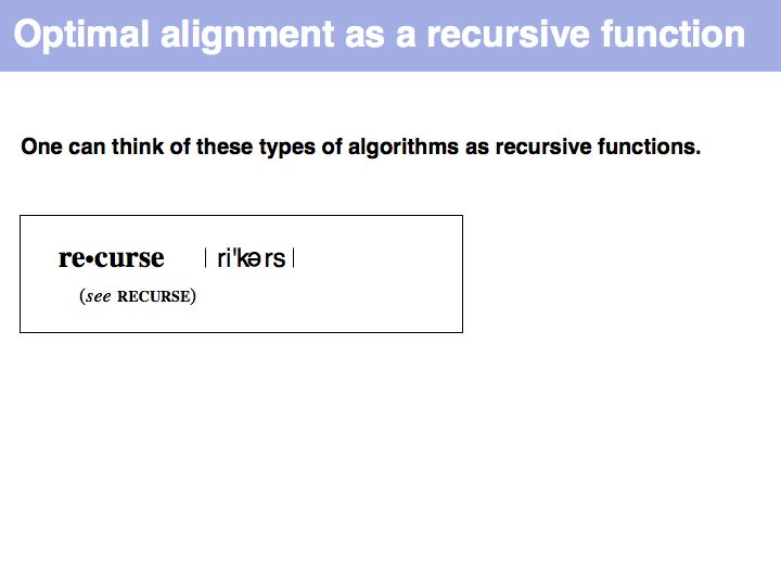
This ironic (!) definition actually defines an infinite recursion - the rule is applied forever.
This ironic (!) definition actually defines an infinite recursion - the rule is applied forever.
Slide 013

Lecture 06, Slide 013
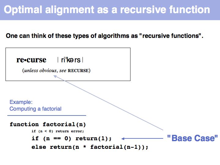
"Real" applications of recursive strategies or algorithms always require a so called Base Case: a situation where the recursion stops and a definite result is generated. More about "Recursion" - read here.
"Real" applications of recursive strategies or algorithms always require a so called Base Case: a situation where the recursion stops and a definite result is generated. More about "Recursion" - read here.
Slide 014

Lecture 06, Slide 014
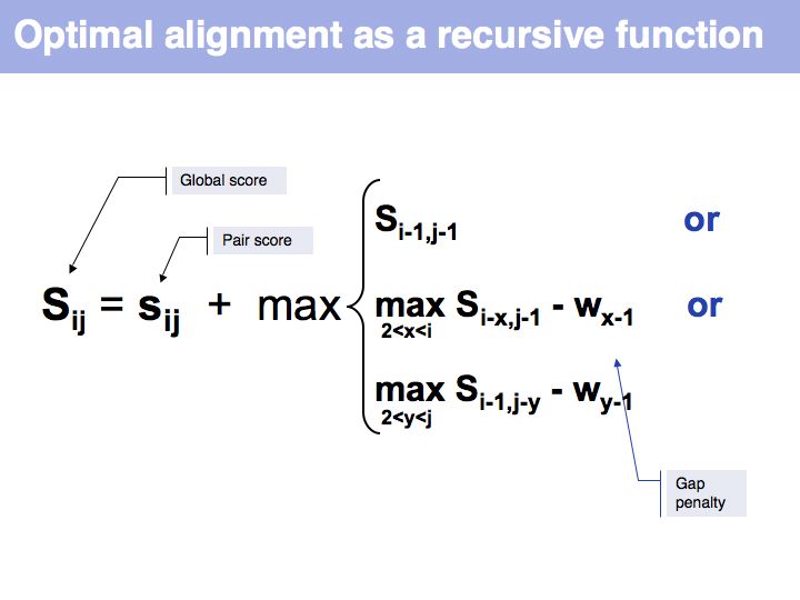
Optimal alignment, in the way we have defined the procedure a few slides ago, is simple to write as a recursion. However, implementing the approach as a recursion is very(!) inefficient since it requires looking up many values several times over. For example if we are to calculate the score for i=9, j=10, we need to consider as one one of the possible extensions the cell i=8, j=9 and x=4 i.e. we need to calculate s8-4,9-1-w4-1 = s4,8-w3. But this is the same value for s we previously had to calculate for the adjacent cell column: i=7, j=9, x=3: s7-3,9-1-w3-1 = s4,8-w2, only with a different w. It is not the w-values that are costly to calculate however, but the s-values themselves, since we need to recurse all the way to the Base Case each time we want to calculate one. So while it is compact to write the alignment in the way given above, in practice we would want to store each intermediate result that is going to be reused. This technique of storing useful intermediate results is called Memoization (not memorization) in computer science.
Optimal alignment, in the way we have defined the procedure a few slides ago, is simple to write as a recursion. However, implementing the approach as a recursion is very(!) inefficient since it requires looking up many values several times over. For example if we are to calculate the score for i=9, j=10, we need to consider as one one of the possible extensions the cell i=8, j=9 and x=4 i.e. we need to calculate s8-4,9-1-w4-1 = s4,8-w3. But this is the same value for s we previously had to calculate for the adjacent cell column: i=7, j=9, x=3: s7-3,9-1-w3-1 = s4,8-w2, only with a different w. It is not the w-values that are costly to calculate however, but the s-values themselves, since we need to recurse all the way to the Base Case each time we want to calculate one. So while it is compact to write the alignment in the way given above, in practice we would want to store each intermediate result that is going to be reused. This technique of storing useful intermediate results is called Memoization (not memorization) in computer science.
The path matrix and the optimal path
Slide 017

Lecture 06, Slide 017
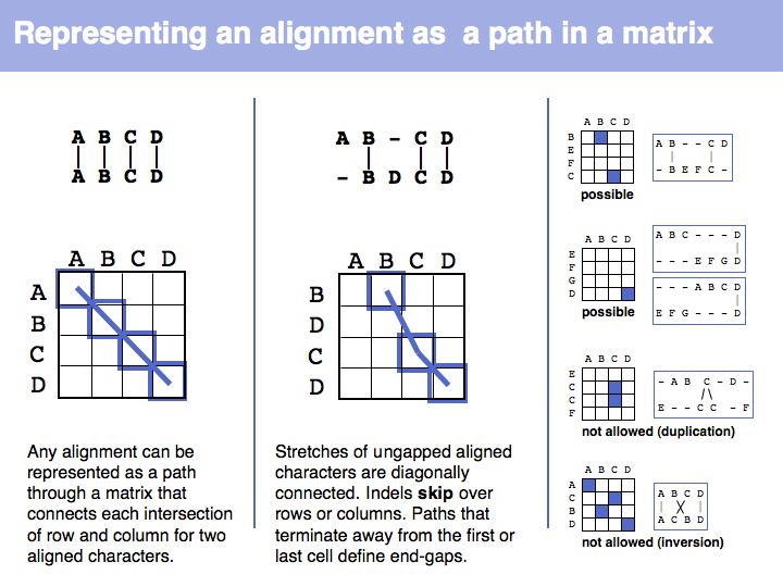
The obvious way to store all intermediate scores for the optimal alignment is in a matrix that has a row for each character of the first sequence, a column for each character of the second. Any alignment can be represented as a path in such a matrix. Only a subset of arrangements correspond to legal paths, corresponding to our usual view of an alignment. However, especially in genome/genome comparisons duplications and inversions are common and specialized algorithms are available to perform such alignments (e.g. Shuffle-LAGAN).
The obvious way to store all intermediate scores for the optimal alignment is in a matrix that has a row for each character of the first sequence, a column for each character of the second. Any alignment can be represented as a path in such a matrix. Only a subset of arrangements correspond to legal paths, corresponding to our usual view of an alignment. However, especially in genome/genome comparisons duplications and inversions are common and specialized algorithms are available to perform such alignments (e.g. Shuffle-LAGAN).
Slide 018

Lecture 06, Slide 018
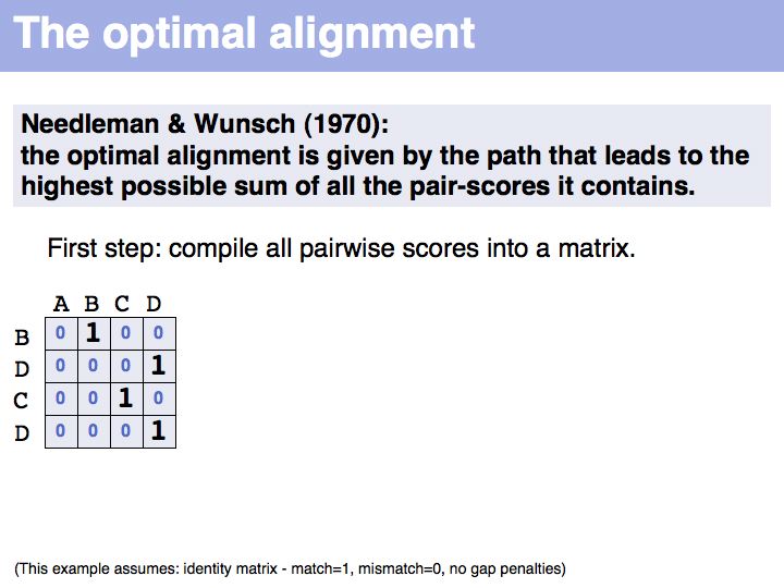
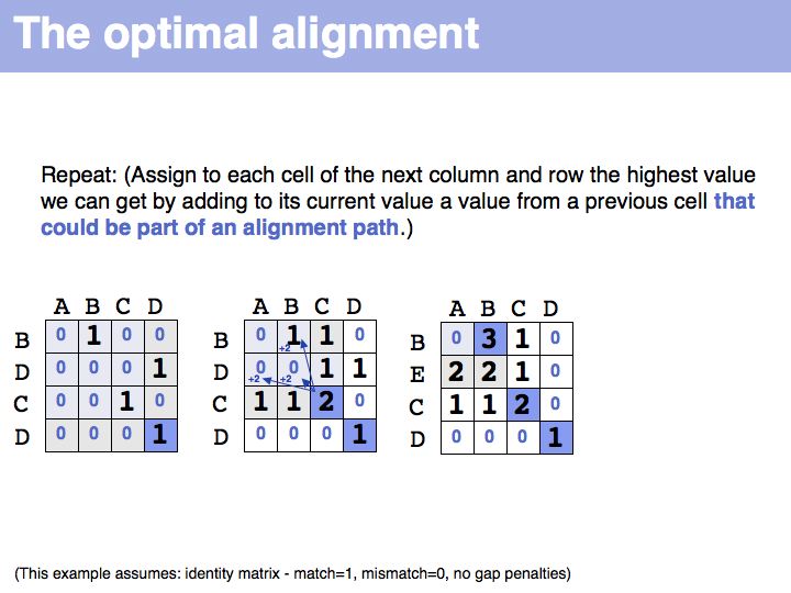
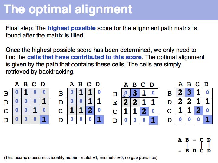
The first step of the Needleman-Wunsch algorithm for global, optimal sequence alignment. This algorithmic strategy is frequently referred to as Dynamic Programming. Here is a link to a larger, explicit example provided by Per Kraulis.
The first step of the Needleman-Wunsch algorithm for global, optimal sequence alignment. This algorithmic strategy is frequently referred to as Dynamic Programming. Here is a link to a larger, explicit example provided by Per Kraulis.
Slide 019

Lecture 06, Slide 019
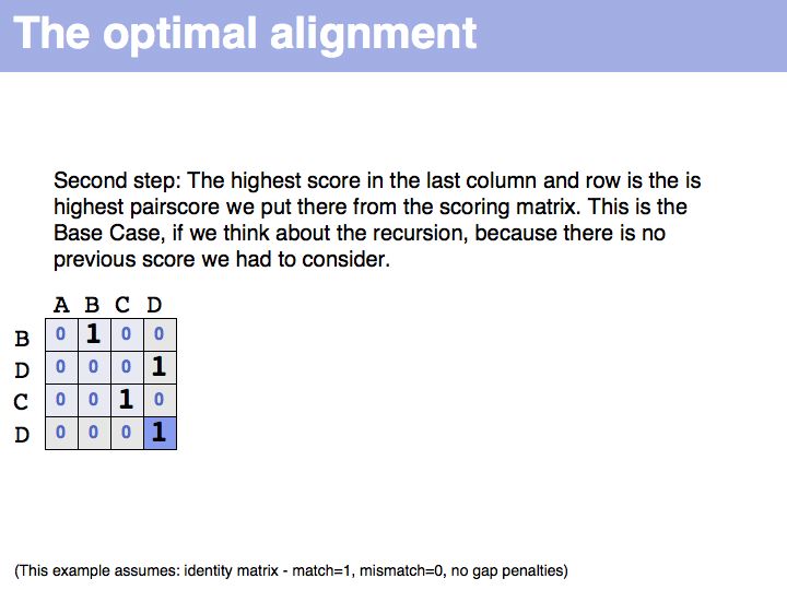
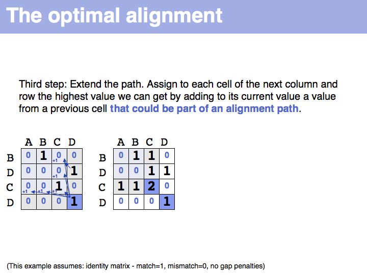
The next scores we need to calculate are the cells in the previous column or row...
The next scores we need to calculate are the cells in the previous column or row...
Slide 020

Lecture 06, Slide 020
Slide 021

Lecture 06, Slide 021
Slide 022

Lecture 06, Slide 022
Slide 023

Lecture 06, Slide 023
Slide 024

Lecture 06, Slide 024
Slide 025

Lecture 06, Slide 025
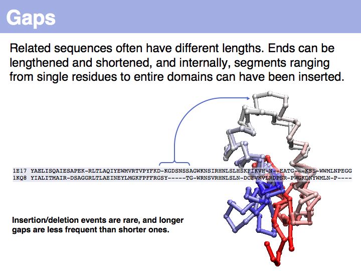
... unfortunately, we have no quantitative, mechanistic model for these events.
... unfortunately, we have no quantitative, mechanistic model for these events.
Slide 026

Lecture 06, Slide 026
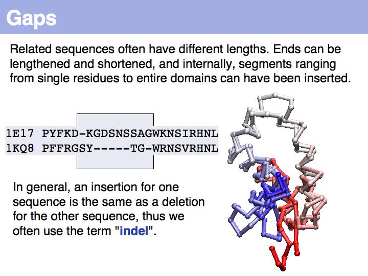
Note that the term insertion or deletion refers only to the sequences, not to the actual molecular event!
Note that the term insertion or deletion refers only to the sequences, not to the actual molecular event!
Slide 027

Lecture 06, Slide 027
Slide 028

Lecture 06, Slide 028
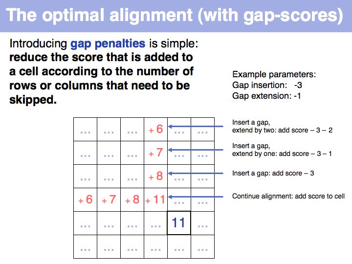
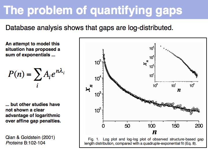
Qian and Goldstein (2001) have shown that a log linear plot of gap probabilities in aligned sequences can be modeled by a sum of four exponential functions. This can be interpreted to mean that several molecular mechanisms could exist for the generation of indels, each with a distinct and characteristic probability of occurrence. However, logarithmic gap penalties do not improve alignments (see Cartwright, 2006 ). Recent developments focus on the inclusion of additional knowledge about the sequences, such as secondary-structure specific gap penalties, or using sequence profiles or multiple alignments, rather than aiming to further improve the gap parameters. The bottom line is: we have no good model for indels, but we have no significantly better model than the simple affine model.
Qian and Goldstein (2001) have shown that a log linear plot of gap probabilities in aligned sequences can be modeled by a sum of four exponential functions. This can be interpreted to mean that several molecular mechanisms could exist for the generation of indels, each with a distinct and characteristic probability of occurrence. However, logarithmic gap penalties do not improve alignments (see Cartwright, 2006 ). Recent developments focus on the inclusion of additional knowledge about the sequences, such as secondary-structure specific gap penalties, or using sequence profiles or multiple alignments, rather than aiming to further improve the gap parameters. The bottom line is: we have no good model for indels, but we have no significantly better model than the simple affine model.
Global and local optimal alignment
Slide 030

Lecture 06, Slide 030
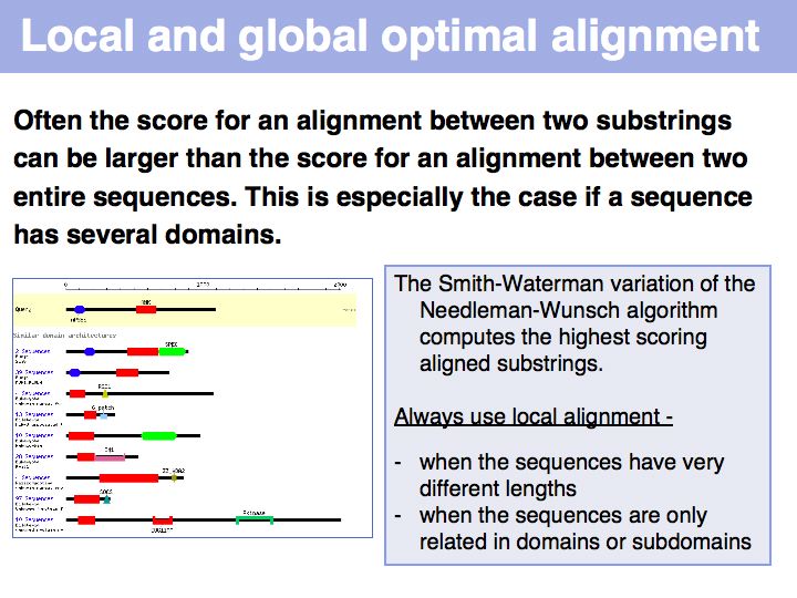
In the example above, the ankyrin domain repeats of the yeast transcription factor Mbp1 are shown as a red box in this graphic of domains in sequence families, compiled in the CDART database. This domain is found in many other proteins, but some of them do not share the other sequence elements found in Mbp1 - they are only partially related. Attempting a global sequence alignment with such sequences would attempt to align sequences that are actually not homologous, leading to inappropriately low scores and the danger of spurios results. http://en.wikipedia.org/wiki/Smith_Waterman_algorithm [Temple Smith and Michael Waterman] have slightly modified the Needleman-Wunsch algorithm, 11 years after its publication, to find the highest scoring local alignment: this is the highest match in the matrix, tracked back to the point where the pathscore drops below zero. The rest of the algorithm works in exactly the same way. There is only one detail that needs to be considered: the substitution matrix must yield a negative expectation value for random alignments. If this were not the case, random pairs could extend the locally high-scoring alignment unreasonably.
In the example above, the ankyrin domain repeats of the yeast transcription factor Mbp1 are shown as a red box in this graphic of domains in sequence families, compiled in the CDART database. This domain is found in many other proteins, but some of them do not share the other sequence elements found in Mbp1 - they are only partially related. Attempting a global sequence alignment with such sequences would attempt to align sequences that are actually not homologous, leading to inappropriately low scores and the danger of spurios results. http://en.wikipedia.org/wiki/Smith_Waterman_algorithm [Temple Smith and Michael Waterman] have slightly modified the Needleman-Wunsch algorithm, 11 years after its publication, to find the highest scoring local alignment: this is the highest match in the matrix, tracked back to the point where the pathscore drops below zero. The rest of the algorithm works in exactly the same way. There is only one detail that needs to be considered: the substitution matrix must yield a negative expectation value for random alignments. If this were not the case, random pairs could extend the locally high-scoring alignment unreasonably.
Slide 031

Lecture 06, Slide 031
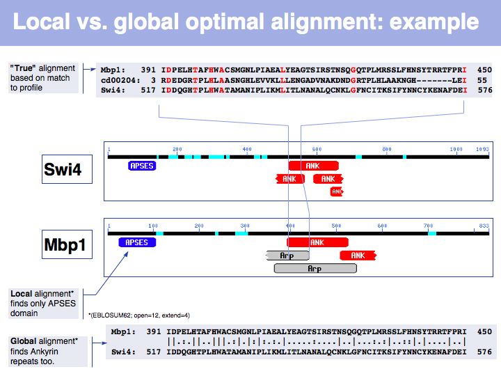
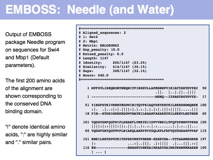
In this example, Smith-Waterman local sequence alignment detects only the high-scoring similarity between Mbp1 and Swi4s APSES domains. The lower scoring, more highly diverged ankyrin repeats are missed by the algorithm. The Needleman-Wunsch alignment finds both sets of sequences, albeit there are segments in between that don't align well at all. In this case, one could do a local alignment, remove the matching segments from the input sequences and then redo the alignment to see if any other significantly similar segments are found.
In this example, Smith-Waterman local sequence alignment detects only the high-scoring similarity between Mbp1 and Swi4s APSES domains. The lower scoring, more highly diverged ankyrin repeats are missed by the algorithm. The Needleman-Wunsch alignment finds both sets of sequences, albeit there are segments in between that don't align well at all. In this case, one could do a local alignment, remove the matching segments from the input sequences and then redo the alignment to see if any other significantly similar segments are found.
Alignment in practice
Slide 033

Lecture 06, Slide 033
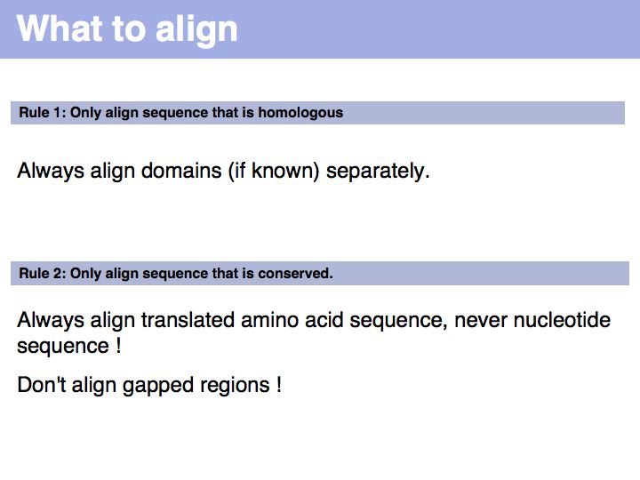
Of course the algorithms will optimally align anything you feed them, but for anything but homologous sequence the alignment will be meaningless. Aligning unrelated sequences is a nice example of cargo-cult bioinformatics. Therefore: if you already know that your proteins are multi-domain, separate out the domains before aligning. If you don't know, critically look at the results, generate a hypothesis about the domain distribution and rerun your alignment from the parts. The exception, of course: is if you know (or believe) your two proteins comprise homologous domains in the same order.
Amino acid sequences are much more highly conserved then genomic sequence and even if you have nucleotide sequences to start from, you should always translate them before aligning. The only reasons to align nucleotides are:
* if you are actually interested in the number of nucleotide exchanges, such as in gene assembly and EST clustering, studies of SNPs, or in comparative genomics, or defining primer binding sites
* if you are aligning untranslated sequences in particular;
* if it is the nucleotide sequence itself that is conserved, such as in DNA binding sites;
* or in RNA genes, such as tRNA or rRNA. A corollary is that you should not try to align sequences in highly gapped regions. These residues have evolved in a non-comparable context, they canot be conserved for that reason and applying our scoring matrices cannot compare such residues in a meaningful way.
Slide 034

Lecture 06, Slide 034
Slide 035

Lecture 06, Slide 035
Slide 036

Lecture 06, Slide 036
Slide 037

Lecture 06, Slide 037
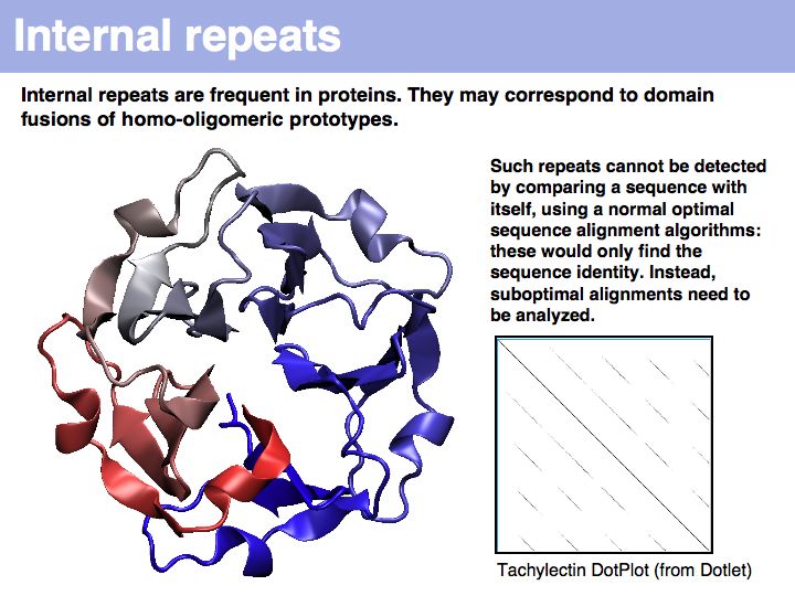
Tachylectin: cherry-blossom symmetry in a lectin from the Japanese horseshoe crab. The dotplot that compares the sequence with itself shows the self-identity matches on the diagonal and five domains, that are all mutually similar (but not identical) to each other as partial similarities on the off-diagonals. If you think of the path matrix as resembling a dotplot, the repeat alignments we need to analyze correspond to the off-diagonal stretches of high similarity.
Tachylectin: cherry-blossom symmetry in a lectin from the Japanese horseshoe crab. The dotplot that compares the sequence with itself shows the self-identity matches on the diagonal and five domains, that are all mutually similar (but not identical) to each other as partial similarities on the off-diagonals. If you think of the path matrix as resembling a dotplot, the repeat alignments we need to analyze correspond to the off-diagonal stretches of high similarity.
Slide 038

Lecture 06, Slide 038
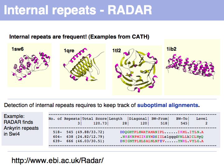
The RADAR server at the EBI analyzes sequences for internal repeats.
The RADAR server at the EBI analyzes sequences for internal repeats.
Slide 039

Lecture 06, Slide 039
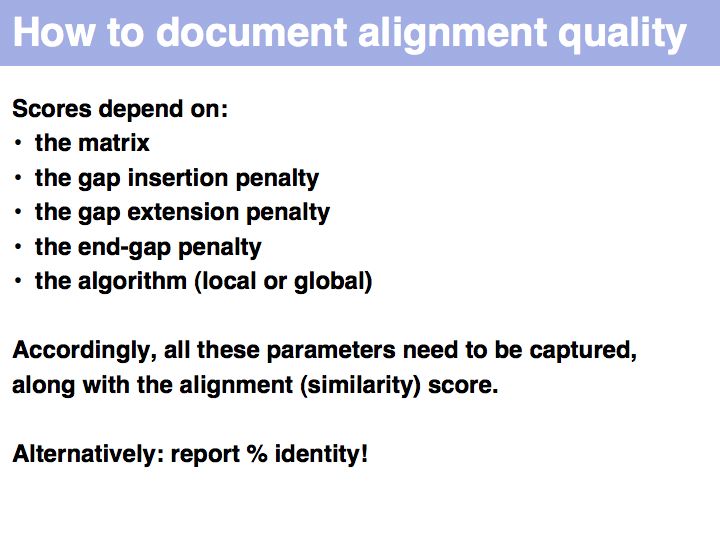
Note that reporting %identity is an objective metric, but it still depends on the exact alignment that has been produced and it does not capture the quality of gaps.
Note that reporting %identity is an objective metric, but it still depends on the exact alignment that has been produced and it does not capture the quality of gaps.
Slide 040

Lecture 06, Slide 040