Lecture 04
Jump to navigation
Jump to search


(Previous lecture) ... (Next lecture)
Sequence Analysis
- What you should take home from this part of the course
- Understand key concepts in probabilistic pattern representation and matching, especially PSSMs. Understand that machine-learning tools such as HMMs (Hidden Markov Models) and NN (Neural Networks) can be used for probabilistic pattern matching and classification.
- Understand the concept of a sequence logo.
- Be familiar with the SignalP Web server.
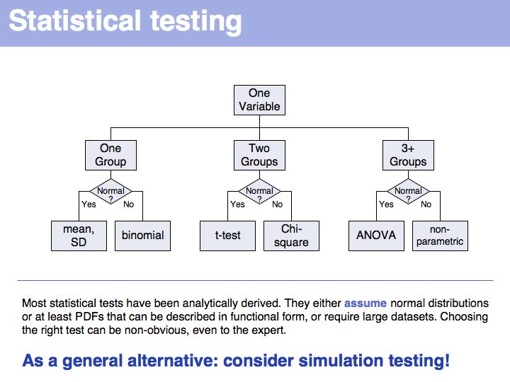
- Know basic concepts of statistics and probability theory, key terms of descriptive statistics;
- Understand probability tables in principle;
- Have encountered important probability distributions;
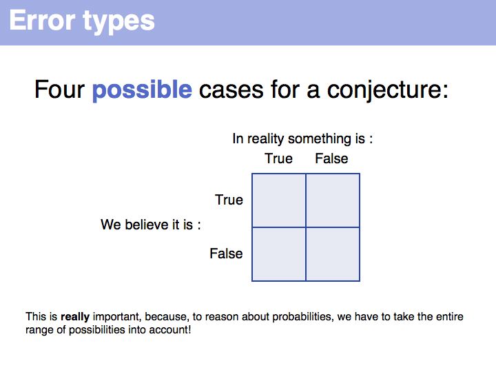
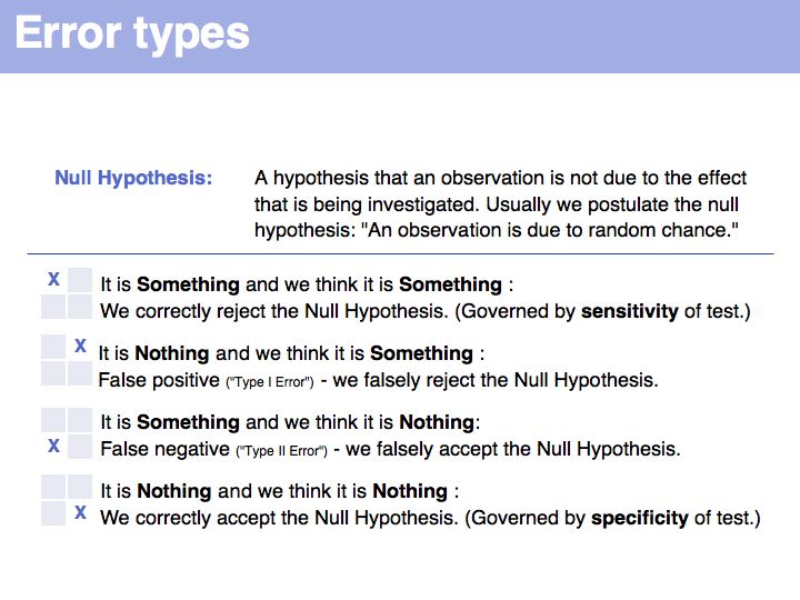
- Understand different error types;
- Understand the terms: significance, confidence interval and statistical test.
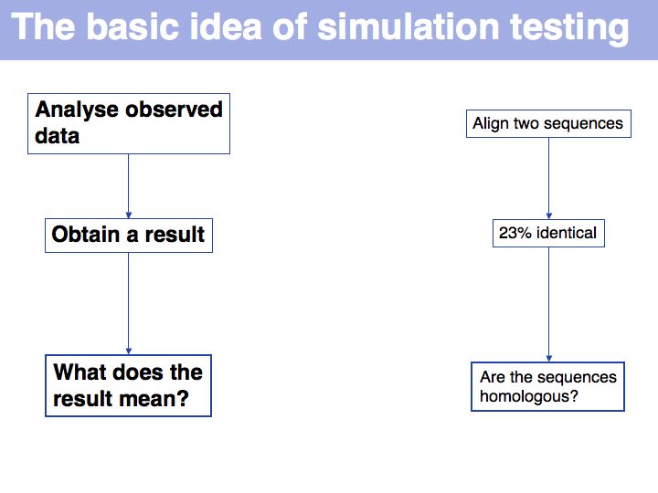
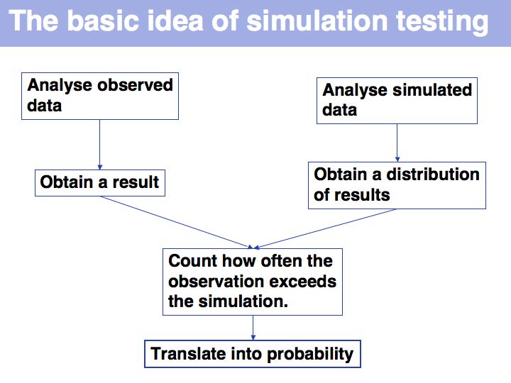
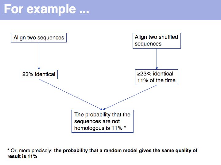
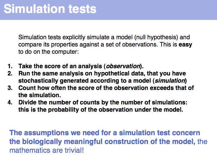
- Be familiar with the concepts and strategy of simulation testing and understand why its simplicity is making an important contribution to computational biology.
- Links summary
- WebLogo
- Tom Schneider's Sequence Logo pages (and introductions to information theory)
- The SignalP server
- Exercises
- If you assume that an 80-mer oligonucleotide can be synthesized with 99.9% coupling efficiency per step and a 0.2% chance of coupling a leftover nucleotide from the previous synthesis step, what is the probability that a randomly picked clone of a gene built with this oligonucleotide has the correct sequence?
- In a recent doctoral thesis defence the candidate claimed that in a microarray expression analysis he was able to show reciprocal regulation of two genes (one related to immune stimulation, the other related to immune suppression): this would mean whenever one gene is regulated up, the other is downregulated, and vice versa. The claim was based on observing this effect in eight of ten experiments. Expression levels were scored semiquantitatively on a scale of (++,+,0,-, and --). Given that such experiments have experimental error as well as biological variability, sketch a simulation test that would analyse whether in fact a significant (anti)correlation had been observed, or whether this result could just as well be due to meaningless fluctuations.
Lecture Slides
Slide 001

Lecture 04, Slide 001
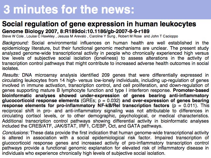
From the Science News, Sept. 14. As far as systems biology complexities go, this one must be near the top: intimate interactions between human's most- and second-most complex systems. The key method here is a bioinformatics approach to classifying genes: pattern searches in the promoter regions. (NB. Not studying in isolation but forming study groups is an excellent idea!). Are you more lonely than average ? Check with the UCLA loneliness scale.
From the Science News, Sept. 14. As far as systems biology complexities go, this one must be near the top: intimate interactions between human's most- and second-most complex systems. The key method here is a bioinformatics approach to classifying genes: pattern searches in the promoter regions. (NB. Not studying in isolation but forming study groups is an excellent idea!). Are you more lonely than average ? Check with the UCLA loneliness scale.
Slide 002

Lecture 04, Slide 002
Slide 003

Lecture 04, Slide 003
Slide 004

Lecture 04, Slide 004
Slide 005

Lecture 04, Slide 005
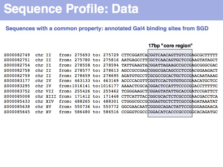
To generate this collection of sequences, the feature "Gal4-binding-site" was searched in the [Saccharomyces Genome Database SGD]; in the resulting overview page binding site annotations recorded by Harbison et al. (2004) were shown for all occurrences; the actual sequences were retrieved by specifying the genome coordinates in the appropriate search form of the database. I have added ten bases upstream and downstream of the core binding region. This procedure could be done by hand in about the same time it took me to write the small screen-scraping program to fetch the sequences. Depending on your programming proficiency, you will find that some tasks can efficiently be done manually, for some tasks it is more efficient to spend the time to search for a better way to achieve them on the Web and only for a comparatively small number of tasks it is worthwhile (or mandatory) to write your own code.
To generate this collection of sequences, the feature "Gal4-binding-site" was searched in the [Saccharomyces Genome Database SGD]; in the resulting overview page binding site annotations recorded by Harbison et al. (2004) were shown for all occurrences; the actual sequences were retrieved by specifying the genome coordinates in the appropriate search form of the database. I have added ten bases upstream and downstream of the core binding region. This procedure could be done by hand in about the same time it took me to write the small screen-scraping program to fetch the sequences. Depending on your programming proficiency, you will find that some tasks can efficiently be done manually, for some tasks it is more efficient to spend the time to search for a better way to achieve them on the Web and only for a comparatively small number of tasks it is worthwhile (or mandatory) to write your own code.
Slide 006

Lecture 04, Slide 006
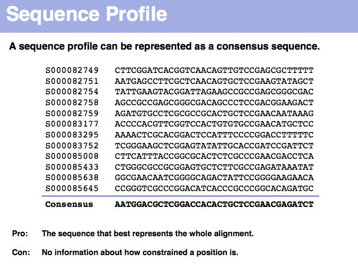
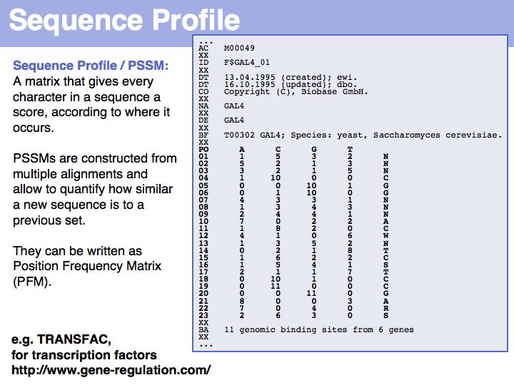
A consensus sequence simply lists the most frequent amino acid or nucleotide at each position, or a random one if there is more than one with the highest frequency. The consensus sequence is the one that you would synthesize to make an idealized representative of the set. It is likely to bind more tightly or to be more stable than each of the individual sequences in the alignment.
A consensus sequence simply lists the most frequent amino acid or nucleotide at each position, or a random one if there is more than one with the highest frequency. The consensus sequence is the one that you would synthesize to make an idealized representative of the set. It is likely to bind more tightly or to be more stable than each of the individual sequences in the alignment.
Slide 007

Lecture 04, Slide 007
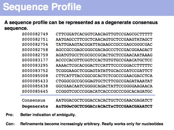
Introducing nucleotide ambiguity codes to represent situations in which more than one nucleotide has the highest frequency improves the situation a bit, but there is also ambiguity. Consider the situation after the conserved CCG pattern: 9 As and 3Gs: should we report the consensusAA, or ist it more interesting to report that the only observed alternative is another purine base and write Y instead?
Introducing nucleotide ambiguity codes to represent situations in which more than one nucleotide has the highest frequency improves the situation a bit, but there is also ambiguity. Consider the situation after the conserved CCG pattern: 9 As and 3Gs: should we report the consensusAA, or ist it more interesting to report that the only observed alternative is another purine base and write Y instead?
Slide 008

Lecture 04, Slide 008
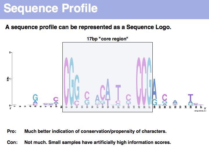
Sequence logo of Gal4 binding sites with 10 nucleotides flanking bases. Created with WebLogo. A Sequence Logo is a graphical representation of aligned sequences where at each position the height of a column is proportional to the (Shannon) information of that position and the relative size of each character is proportional to its frequency within the column. Sequence Logos were pioneered by Tom Schneider who maintains an informative Website about their use and theoretical foundations. Note that there is considerable additional information in the flanking sequences that are not included in the published description of the core binding pattern; it is advantageous if you are able to rerun such analyses, rather than rely on someone else's opinion.
Sequence logo of Gal4 binding sites with 10 nucleotides flanking bases. Created with WebLogo. A Sequence Logo is a graphical representation of aligned sequences where at each position the height of a column is proportional to the (Shannon) information of that position and the relative size of each character is proportional to its frequency within the column. Sequence Logos were pioneered by Tom Schneider who maintains an informative Website about their use and theoretical foundations. Note that there is considerable additional information in the flanking sequences that are not included in the published description of the core binding pattern; it is advantageous if you are able to rerun such analyses, rather than rely on someone else's opinion.
Slide 009

Lecture 04, Slide 009
Slide 010

Lecture 04, Slide 010
Slide 011

Lecture 04, Slide 011
Since log(0) is not defined, we have to introduce an arbitrary correction for unobserved characters. In this example I have simply added 0.1 to each character frequency before calculating log odds.
Since log(0) is not defined, we have to introduce an arbitrary correction for unobserved characters. In this example I have simply added 0.1 to each character frequency before calculating log odds.
Slide 012

Lecture 04, Slide 012
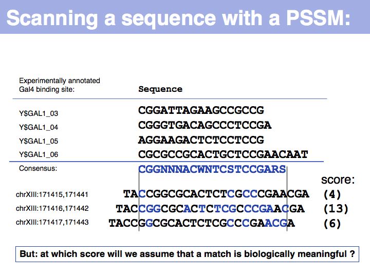
In this informal example, I have simply counted matches with the consensus sequence (excluding "N"). We can slide the PSSM over the entire chromosome, and calculate scores for each position. Only the middle sequence is an annotated binding site. Whatever method we use for probabilistic pattern matching, we will always get a score. It is then our problem to decide what the score means.
In this informal example, I have simply counted matches with the consensus sequence (excluding "N"). We can slide the PSSM over the entire chromosome, and calculate scores for each position. Only the middle sequence is an annotated binding site. Whatever method we use for probabilistic pattern matching, we will always get a score. It is then our problem to decide what the score means.
Slide 013

Lecture 04, Slide 013
Slide 014

Lecture 04, Slide 014
Slide 015

Lecture 04, Slide 015
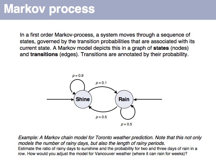
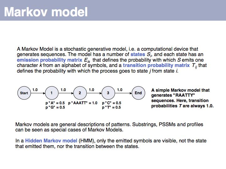
This first order Markov model depends only on the current state. Higher-order models take increasing lengths of "history" into account, how the system arrived in its current state. Note that the exit probabilities fo a state always have to sum to 1.0. The so called "stationary probability" over a long period of time for p(rain) is 0.167 - this is determined by the combined effects of all individual transition probabilities. The stationary probabilities for two- or three consecutive rainy days are 4.2% and 2.1%, respectively.
This first order Markov model depends only on the current state. Higher-order models take increasing lengths of "history" into account, how the system arrived in its current state. Note that the exit probabilities fo a state always have to sum to 1.0. The so called "stationary probability" over a long period of time for p(rain) is 0.167 - this is determined by the combined effects of all individual transition probabilities. The stationary probabilities for two- or three consecutive rainy days are 4.2% and 2.1%, respectively.
Slide 016

Lecture 04, Slide 016
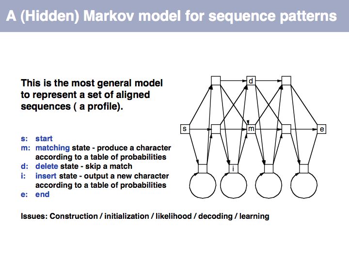
Hidden Markov Model: on Wikipedia.
Hidden Markov Model: on Wikipedia.
Slide 017

Lecture 04, Slide 017
Slide 018

Lecture 04, Slide 018
Slide 019

Lecture 04, Slide 019
Slide 020

Lecture 04, Slide 020
Slide 021

Lecture 04, Slide 021
Slide 022

Lecture 04, Slide 022
Slide 023

Lecture 04, Slide 023
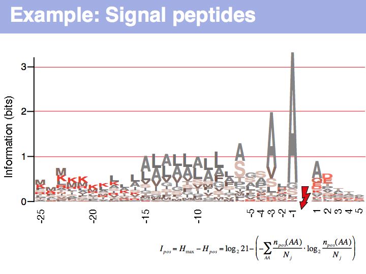
Signal peptide example for recognition of sequence features with HMMs or NNs: common features in gram-negative signal-peptide sequences are shown in a Sequence Logo. Sequences were aligned on the signal-peptidase cleavage site. Their common features include a positively charged N-terminus, a hydrophobic helical stretch and a small residue that precedes the actual cleavage site.
Signal peptide example for recognition of sequence features with HMMs or NNs: common features in gram-negative signal-peptide sequences are shown in a Sequence Logo. Sequences were aligned on the signal-peptidase cleavage site. Their common features include a positively charged N-terminus, a hydrophobic helical stretch and a small residue that precedes the actual cleavage site.
Slide 024

Lecture 04, Slide 024
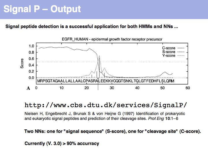
SignalP is the premier Web server to detect signal sequences.
SignalP is the premier Web server to detect signal sequences.
Slide 025

Lecture 04, Slide 025
Slide 026

Lecture 04, Slide 026
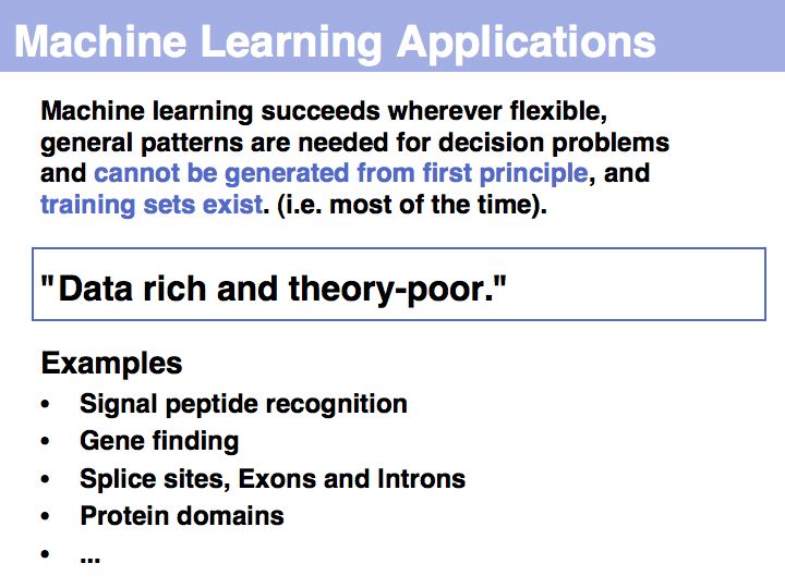
... however: machine learning will find correlations, not causalities. It cannot replace your biological insight to distinguish a statistical anomaly from a biologically meaningful result!
... however: machine learning will find correlations, not causalities. It cannot replace your biological insight to distinguish a statistical anomaly from a biologically meaningful result!
Slide 027
deleted
Slide 028

Lecture 04, Slide 028
Slide 029

Lecture 04, Slide 029
Slide 030

Lecture 04, Slide 030
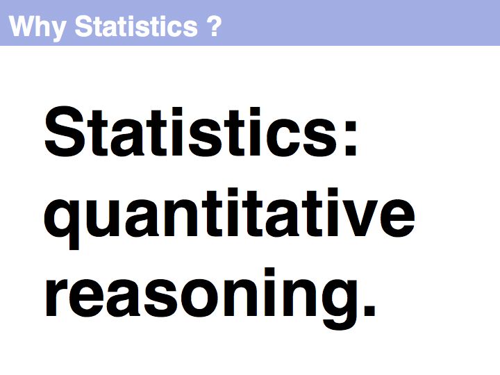
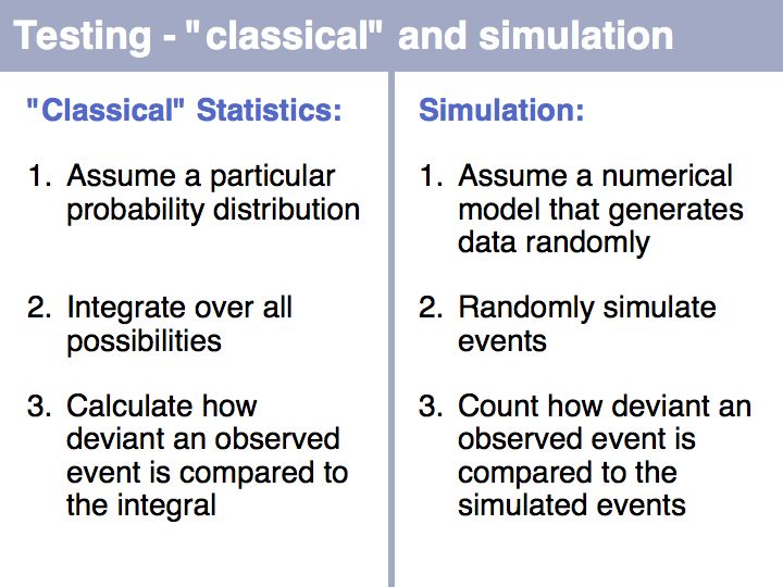
This is why statistics is cool.
This is why statistics is cool.
Slide 031

Lecture 04, Slide 031
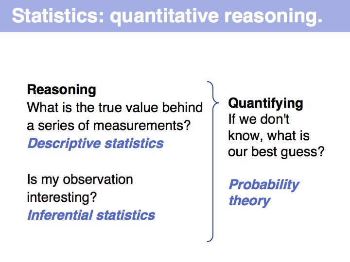
The distinction is somewhat artificial in practice: parameter estimations from probability theory can be excellent descriptors!
The distinction is somewhat artificial in practice: parameter estimations from probability theory can be excellent descriptors!
Slide 032

Lecture 04, Slide 032
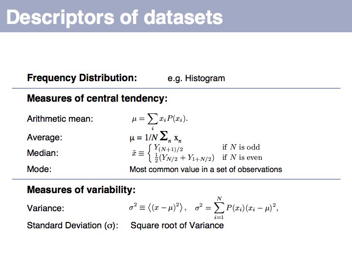
You should be familiar with these most fundamental descriptors, they come up time- and time again in the literature. Here is a series of highly readable reviews on topics of medical statistics by Jonathan Ball and Coauthors:
*(1)Presenting and summarising data
*(2) Samples and populations
*(3) Hypothesis testing and P values
*(4) Sample size calculations
*(5) Comparison of means
*(6) Nonparametric methods
*(7) Correlation and regression
*(8) Qualitative data - tests of association
*(9) One-way analysis of variance
*(10) Further nonparametric methods
*(11) Assessing risk
*(12) Survival analysis
*(13) Receiver operating characteristic curves
*(14) Logistic regression
Slide 033

Lecture 04, Slide 033
Slide 034

Lecture 04, Slide 034
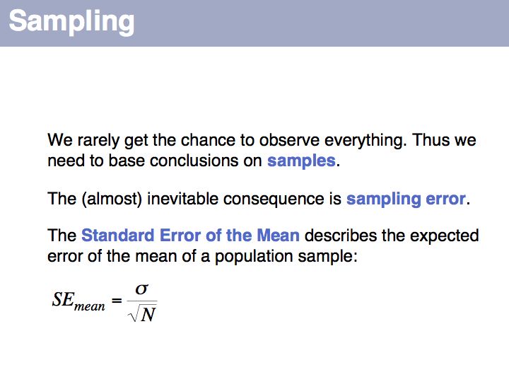
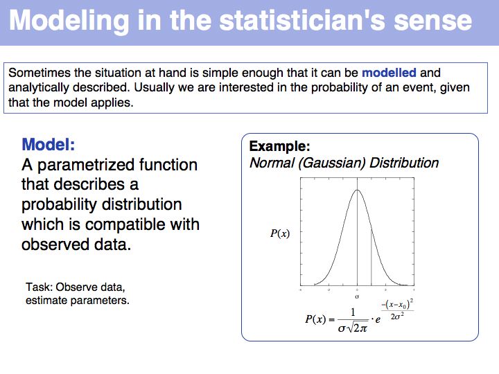
Statistical model: on Wikipedia.
Statistical model: on Wikipedia.
Slide 035

Slide 036

Lecture 04, Slide 036
(*) Worst error in the clipart: no two faces of a die have the same number of dots. Three more errors: opposing sides must add to seven. The ones should be at the bottom if the sixes face up.
(*) Worst error in the clipart: no two faces of a die have the same number of dots. Three more errors: opposing sides must add to seven. The ones should be at the bottom if the sixes face up.
Slide 037

Lecture 04, Slide 037
Slide 038

Lecture 04, Slide 038
Slide 039

Lecture 04, Slide 039
Slide 040

Lecture 04, Slide 040
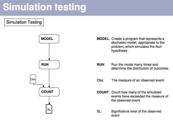
Still not convinced? Try the simulation here.
Still not convinced? Try the simulation here.
Slide 041

Slide 042

Slide 043

Slide 044

Slide 045

Slide 046

Slide 047

Slide 048

Lecture 04, Slide 048
Slide 049

Lecture 04, Slide 049
Don't use: Type I error - say "False positive". Don't use: Type II error - say "False negative".
Don't use: Type I error - say "False positive". Don't use: Type II error - say "False negative".
Slide 050

Slide 051

Slide 052

Lecture 04, Slide 052
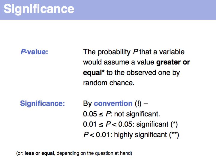
Note that a P-value is not the probability of a particular event occurring - that probability could be arbitrarily small, depending on the resolution of the measurement. It is the probability that an event occurs that is equal to or larger than the observed one.
Note that a P-value is not the probability of a particular event occurring - that probability could be arbitrarily small, depending on the resolution of the measurement. It is the probability that an event occurs that is equal to or larger than the observed one.
Slide 053

Slide 054

Lecture 04, Slide 054
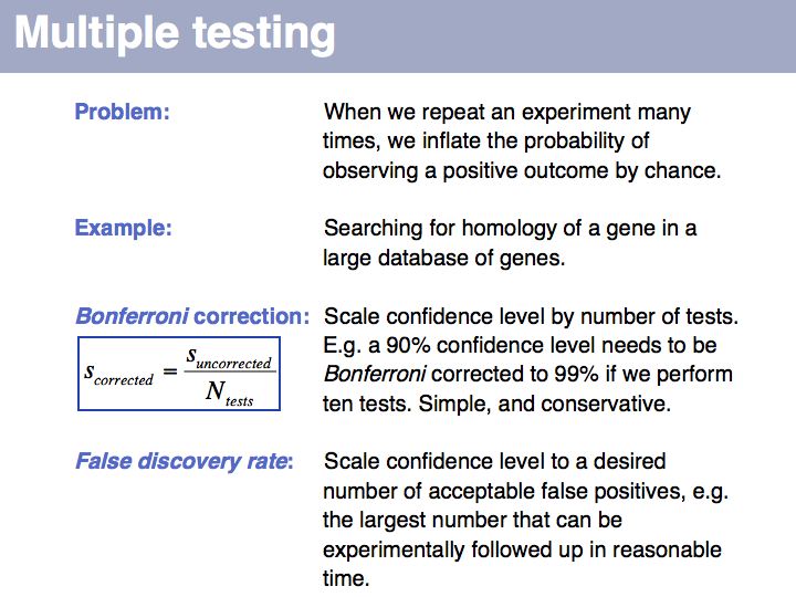
Multiple testing: on Wikipedia
Multiple testing: on Wikipedia
Slide 055

Lecture 04, Slide 055
Slide 056

Slide 057

Lecture 04, Slide 057
Slide 058

Lecture 04, Slide 058
Slide 059

Lecture 04, Slide 059
Slide 060

Lecture 04, Slide 060
Slide 061

Lecture 04, Slide 061
Slide 062

Lecture 04, Slide 062
Slide 063

Lecture 04, Slide 063
Slide 064

Slide 065

Lecture 04, Slide 065
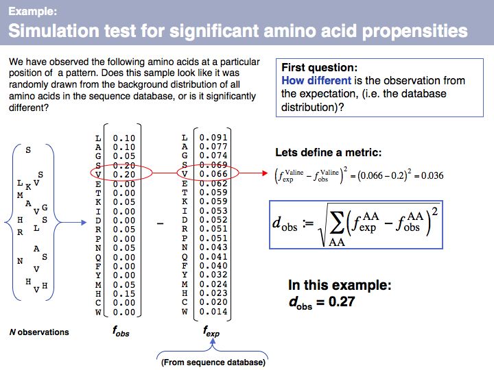
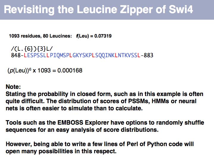
We can describe a set of observations as a distribution, and we can express this distribution as a vector if we define each element of the vector to represent a particular amino acid. This gives us a convenient and intuitive way to define a metric to compare two distributions - by considering the difference between all components of the two distributions. If we interpret this geometrically, the distribution of n-elements corresponds to a point in an n-dimensional spaceand the difference we are using here is the distance between the two points defined by the two distributions. We could use different metrics, but this one (the vector norm) is intuitive and convenient. The comparison between the frequency distribution of all amino acids in the sequence database (fexp, the expected distribution for a random sample of amino acids )
We can describe a set of observations as a distribution, and we can express this distribution as a vector if we define each element of the vector to represent a particular amino acid. This gives us a convenient and intuitive way to define a metric to compare two distributions - by considering the difference between all components of the two distributions. If we interpret this geometrically, the distribution of n-elements corresponds to a point in an n-dimensional spaceand the difference we are using here is the distance between the two points defined by the two distributions. We could use different metrics, but this one (the vector norm) is intuitive and convenient. The comparison between the frequency distribution of all amino acids in the sequence database (fexp, the expected distribution for a random sample of amino acids )
Slide 066

Lecture 04, Slide 066
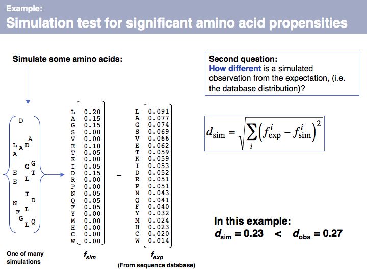
We can apply the same metric to a set of the same number of simulated amino acids, in which the probability of picking an amino acid is given by its expectation value, fexp. If we do this many times, we will obtain a distribution of d values that tells us how different the relative frequencies of amino acids are, when they are generated by our simulator, relative to what we see in the database. Note that under many simulations we still gat an error every time, simply because the number of amino acids in every single run is small (20, in our example) and thus do what we want, the sample can never exactly reproduce the database distribution. This is important to understand: we are not simulating the distribution, we are simulating the influence of a limited-size sample!
We can apply the same metric to a set of the same number of simulated amino acids, in which the probability of picking an amino acid is given by its expectation value, fexp. If we do this many times, we will obtain a distribution of d values that tells us how different the relative frequencies of amino acids are, when they are generated by our simulator, relative to what we see in the database. Note that under many simulations we still gat an error every time, simply because the number of amino acids in every single run is small (20, in our example) and thus do what we want, the sample can never exactly reproduce the database distribution. This is important to understand: we are not simulating the distribution, we are simulating the influence of a limited-size sample!
Slide 067

Lecture 04, Slide 067
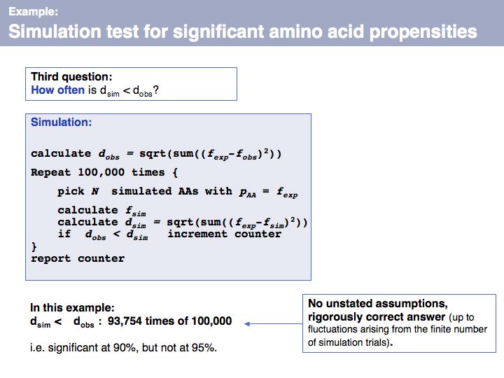
Once we have simulated the experiment many times, we can compare the observed outcome with the one that would be expected if the amino acids had been randomly picked from a database distribution. In our example, the result deviates considerably from what we would expect, but not as much so that it meet a significance level of 95%.
Once we have simulated the experiment many times, we can compare the observed outcome with the one that would be expected if the amino acids had been randomly picked from a database distribution. In our example, the result deviates considerably from what we would expect, but not as much so that it meet a significance level of 95%.
Slide 068

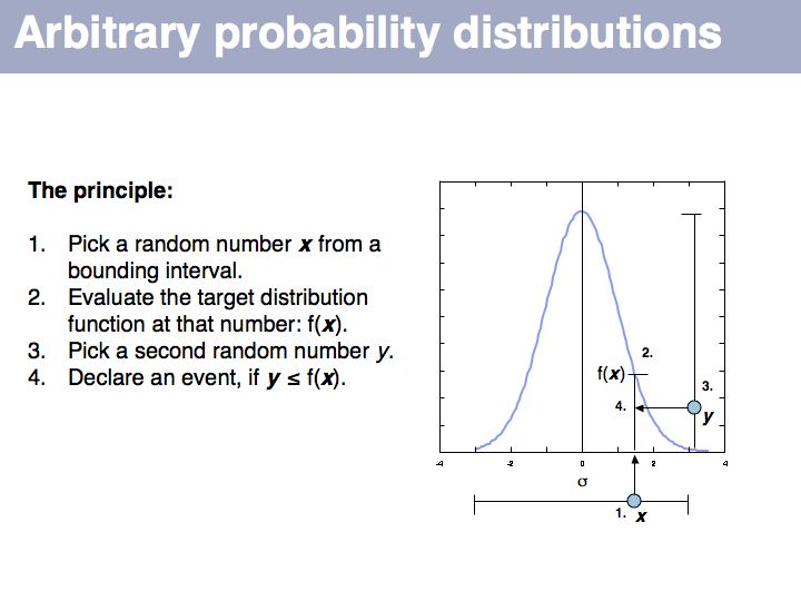
. Standard random number generators generate uniformly distributed random numbers. Thus when you check into which interval one has fallen, this designates a choice with the right target probability so in that interval will then pick a
Slide 069

Lecture 04, Slide 069
If we want to simulate events according to a particular probability distribution, we can use the procedure given above. The procedure is not very efficient, since many values will be discarded if the interval is large. For each particular distribution there will be more efficient, specialized ways to generate it. However this procedure is completely general and it is trivial to change the target probability distribution's parameters; all you need is the definition of the distribution.
If we want to simulate events according to a particular probability distribution, we can use the procedure given above. The procedure is not very efficient, since many values will be discarded if the interval is large. For each particular distribution there will be more efficient, specialized ways to generate it. However this procedure is completely general and it is trivial to change the target probability distribution's parameters; all you need is the definition of the distribution.
Slide 070

Lecture 04, Slide 070
Slide 071

Lecture 04, Slide 071
Slide 072

Lecture 04, Slide 072
Slide 073

Lecture 04, Slide 073
Slide 074

Lecture 04, Slide 074
Slide 075

Lecture 04, Slide 075