Storing Data

Contents
Store Data
- A protein datamodel
- Implementing the Data Model in R
Report topic
Further Reading
Questions, comments
References

Expected Preparations:

	[BIN] Abstractions
	The units listed above are part of this course and contain important preparatory material.

Keywords: Representation of data; common data formats; implementing a data model; JSON

Objectives:

This unit will …

Introduce principles of storing data in different formats and principles of supporting storage, maintenance, and retrieval with different tools;
Implement relational data models as lists of data frames in R;
Develop code for this purpose and teach how to work with such code;
Find the closest homologue of Mbp1 in MYSPE.

Outcomes:

After working through this unit you …

can recommend alternatives for storing data, depending on the context and objectives;
can create, edit and validate JSON formatted data;
have practiced creating a relational database as a list of dataframes;
can query the database directly, and via cross-referencing tables;
have discovered the closest homologue to yeast Mbp1 in MYSPE;
have added key information about this protein to the database;

Deliverables:

Time management: Before you begin, estimate how long it will take you to complete this unit. Then, record in your course journal: the number of hours you estimated, the number of hours you worked on the unit, and the amount of time that passed between start and completion of this unit.

Journal: Document your progress in your Course Journal. Some tasks may ask you to include specific items in your journal. Don’t overlook these.

Insights: If you find something particularly noteworthy about this unit, make a note in your insights! page.

Your protein database Write a database-generating script that loads a protein database from JSON files.

Evaluation:

Material based on this learning unit can be submitted for formative feedback. To submit:

Create a new document in your shared Google drive folder.
Call your document BIN-Storing_Data-<your name>-2022
Write a short report on the topic defined below.
Include a (CC) license at the end of your document, as instructed at the beginning of the course.
When you are done with everything, go to the Assignments page on Quercus and open the first Feedback Unit that you have not submitted yet. Paste the URL of your report document into the form, and click on Submit Assignment. Your link can be submitted only once and not edited. Also: do not edit your document after it has been submitted.

If your report includes R code …

… then please follow these additional instructions.

Submitted R code must be placed into a code appendix.
We will load the code for evaluation. Therefore the code in your appendix must be delimited with two special tags.
- The first line of your code must be
  # begin code
- The last line must be
  # end code
- Use only these tags and make sure they appear only once in your document.
The second line of your code must be a comment that identifies you as the author and the title of your report.
You can run fetchGoogleDocRcode(<your doc URL>) to check that your code can be loaded into R.
The submitted code must be exactly the code that you have used to obtain your results. Altering the code in your documentation - even if only for cosmetic purposes - is an academic offence.
The reported results must be exactly the results your code has produced at the time you ran it. Altering the results you obtained - for any reason whatsoever - is an academic offence.
It must be possible to reproduce your exact results from your posted code. Therefore:
- Make sure your code is complete and can stand alone when we run it. All data and other assets must be included with the code.
- Do not create or delete files in your code.
- If you need special R packages, only packages from CRAN or BioConductor may be used.
- Use set.seed(<some integer>) for reproducible randomness wherever appropriate (and verify that your results can be reproduced).

Please remember that code submissions have their own marking rubrics.

This unit discusses options for storing and organizing data in a variety of formats, and develops R code for a protein data model, based on JSON formatted source data.

Task…

Read the introductory notes on concepts about storing data for bioinformaticsPDF.

Any software project requires modelling on many levels - data-flow models, logic models, user interaction models and more. But all of these ultimately rely on a data model that defines how the world is going to be represented in the computer for the project’s purpose. The process of abstraction of data entities and defining their relationships can (and should) take up a major part of the project definition, often taking several iterations until you get it right. Whether your data can be completely described, consistently stored and efficiently retrieved is determined to a large part by your data model.

Databases(W) can take many forms, from memories in your brain, to shoe-cartons under your bed, to software applications on your computer, or warehouse-sized data centres. Fundamentally, these all do the same thing: collect information and make it available for retrieval.

Let us consider collecting information on APSES-domain transcription factors in various fungi, with the goal of being able to compare the transcription factors. Let’s specify this as follows:

Store data on APSES-domain proteins so that we can

cross reference the source databases;
study if they have the same features (e.g. domains);
and compare the features across species.

The underlying information can easily be retrieved for a protein from its RefSeq or UniProt entry.

Text files

A first attempt to organize the data might be simply to write it down as text:

name: Mbp1
refseq ID: NP_010227
uniprot ID: P39678
species: Saccharomyces cerevisiae
taxonomy ID: 4392
sequence:
MSNQIYSARYSGVDVYEFIHSTGSIMKRKKDDWVNATHILKAANFAKAKR
TRILEKEVLKETHEKVQGGFGKYQGTWVPLNIAKQLAEKFSVYDQLKPLF
DFTQTDGSASPPPAPKHHHASKVDRKKAIRSASTSAIMETKRNNKKAEEN
QFQSSKILGNPTAAPRKRGRPVGSTRGSRRKLGVNLQRSQSDMGFPRPAI
PNSSISTTQLPSIRSTMGPQSPTLGILEEERHDSRQQQPQQNNSAQFKEI
DLEDGLSSDVEPSQQLQQVFNQNTGFVPQQQSSLIQTQQTESMATSVSSS
PSLPTSPGDFADSNPFEERFPGGGTSPIISMIPRYPVTSRPQTSDINDKV
NKYLSKLVDYFISNEMKSNKSLPQVLLHPPPHSAPYIDAPIDPELHTAFH
WACSMGNLPIAEALYEAGTSIRSTNSQGQTPLMRSSLFHNSYTRRTFPRI
FQLLHETVFDIDSQSQTVIHHIVKRKSTTPSAVYYLDVVLSKIKDFSPQY
RIELLLNTQDKNGDTALHIASKNGDVVFFNTLVKMGALTTISNKEGLTAN
EIMNQQYEQMMIQNGTNQHVNSSNTDLNIHVNTNNIETKNDVNSMVIMSP
VSPSDYITYPSQIATNISRNIPNVVNSMKQMASIYNDLHEQHDNEIKSLQ
KTLKSISKTKIQVSLKTLEVLKESSKDENGEAQTNDDFEILSRLQEQNTK
KLRKRLIRYKRLIKQKLEYRQTVLLNKLIEDETQATTNNTVEKDNNTLER
LELAQELTMLQLQRKNKLSSLVKKFEDNAKIHKYRRIIREGTEMNIEEVD
SSLDVILQTLIANNNKNKGAEQIITISNANSHA
length: 833
Kila-N domain: 21-93
Ankyrin domains: 369-455, 505-549

...

… and save it all in one large text file and whenever you need to look something up, you just open the file, look for e.g. the name of the protein and read what’s there. Or - for a more structured approach, you could put this into several files in a folder.¹ This is a perfectly valid approach and for some applications it might not be worth the effort to think more deeply about how to structure the data, and store it in a way that it is robust and scales easily to large datasets. Alas, small projects have a tendency to grow into large projects and if you work in this way, it’s almost guaranteed that you will end up doing many things by hand that could easily be automated. Imagine asking questions like:

How many proteins do I have?
What’s the sequence of the Kila-N domain?
What percentage of my proteins have an Ankyrin domain?
Or two …?

Answering these questions “by hand” is possible, but tedious.

Spreadsheets

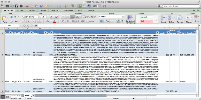
Data for three yeast APSES domain proteins in an Excel spreadsheet. (DB_Excel-spreadsheet.jpg)

Many serious researchers keep their project data in spreadsheets. Often they use Excel, or an alternative like the free OpenOffice Calc, or Google Sheets, both of which are compatible with Excel and have some interesting advantages. Here, all your data is in one place, easy to edit. You can even do simple calculations - although you should never use Excel for statistics². You could answer What percentage of my proteins have an Ankyrin domain? quite easily³.

There are two major downsides to spreadsheets. For one, complex queries require programming. There is no way around this. You can program inside Excel with Visual Basic. But you might as well export your data so you can work on it with a “real” programming language. The other thing is that Excel does not scale very well. Once you have more than a hundred proteins in your spreadsheet, you can see how finding anything can become tedious.

However, just because Excel was built for business applications, and designed for use by office assistants, does not mean it is intrinsically unsuitable for our domain. It’s important to be pragmatic, not dogmatic, when choosing tools: choose according to your real requirements. Sometimes “quick and dirty” is just fine, because quick.

R

R can keep complex data in data frames and lists. If we do data analysis with R, we have to load the data first. We can use any of the read.table() functions for structured data, read lines of raw text with readLines(), or slurp in entire files with scan(). Convenient packages exist to parse structured data like XML or JSON and import it. But we could also keep the data in an R object in the first place that we can read from disk, analyze, modify, and write back. In this case, R becomes our database engine.

# Sample construction of an R database table as a dataframe

# Data for the Mbp1 protein
proteins <- data.frame(
    name     = "Mbp1",
    refSeq   = "NP_010227",
    uniProt  = "P39678",
    species  = "Saccharomyces cerevisiae",
    taxId    = "4392",
    sequence = paste(
                    "MSNQIYSARYSGVDVYEFIHSTGSIMKRKKDDWVNATHILKAANFAKAKR",
                    "TRILEKEVLKETHEKVQGGFGKYQGTWVPLNIAKQLAEKFSVYDQLKPLF",
                    "DFTQTDGSASPPPAPKHHHASKVDRKKAIRSASTSAIMETKRNNKKAEEN",
                    "QFQSSKILGNPTAAPRKRGRPVGSTRGSRRKLGVNLQRSQSDMGFPRPAI",
                    "PNSSISTTQLPSIRSTMGPQSPTLGILEEERHDSRQQQPQQNNSAQFKEI",
                    "DLEDGLSSDVEPSQQLQQVFNQNTGFVPQQQSSLIQTQQTESMATSVSSS",
                    "PSLPTSPGDFADSNPFEERFPGGGTSPIISMIPRYPVTSRPQTSDINDKV",
                    "NKYLSKLVDYFISNEMKSNKSLPQVLLHPPPHSAPYIDAPIDPELHTAFH",
                    "WACSMGNLPIAEALYEAGTSIRSTNSQGQTPLMRSSLFHNSYTRRTFPRI",
                    "FQLLHETVFDIDSQSQTVIHHIVKRKSTTPSAVYYLDVVLSKIKDFSPQY",
                    "RIELLLNTQDKNGDTALHIASKNGDVVFFNTLVKMGALTTISNKEGLTAN",
                    "EIMNQQYEQMMIQNGTNQHVNSSNTDLNIHVNTNNIETKNDVNSMVIMSP",
                    "VSPSDYITYPSQIATNISRNIPNVVNSMKQMASIYNDLHEQHDNEIKSLQ",
                    "KTLKSISKTKIQVSLKTLEVLKESSKDENGEAQTNDDFEILSRLQEQNTK",
                    "KLRKRLIRYKRLIKQKLEYRQTVLLNKLIEDETQATTNNTVEKDNNTLER",
                    "LELAQELTMLQLQRKNKLSSLVKKFEDNAKIHKYRRIIREGTEMNIEEVD",
                    "SSLDVILQTLIANNNKNKGAEQIITISNANSHA",
                    sep=""),
    seqLen   = 833,
    KilAN    = "21-93",
    Ankyrin  = "369-455, 505-549")

# add data for the Swi4 protein
proteins <- rbind(proteins,
                  data.frame(
    name     = "Swi4",
    refSeq   = "NP_011036",
    uniProt  = "P25302",
    species  = "Saccharomyces cerevisiae",
    taxId    = "4392",
    sequence = paste(
                    "MPFDVLISNQKDNTNHQNITPISKSVLLAPHSNHPVIEIATYSETDVYEC",
                    "YIRGFETKIVMRRTKDDWINITQVFKIAQFSKTKRTKILEKESNDMQHEK",
                    "VQGGYGRFQGTWIPLDSAKFLVNKYEIIDPVVNSILTFQFDPNNPPPKRS",
                    "KNSILRKTSPGTKITSPSSYNKTPRKKNSSSSTSATTTAANKKGKKNASI",
                    "NQPNPSPLQNLVFQTPQQFQVNSSMNIMNNNDNHTTMNFNNDTRHNLINN",
                    "ISNNSNQSTIIQQQKSIHENSFNNNYSATQKPLQFFPIPTNLQNKNVALN",
                    "NPNNNDSNSYSHNIDNVINSSNNNNNGNNNNLIIVPDGPMQSQQQQQHHH",
                    "EYLTNNFNHSMMDSITNGNSKKRRKKLNQSNEQQFYNQQEKIQRHFKLMK",
                    "QPLLWQSFQNPNDHHNEYCDSNGSNNNNNTVASNGSSIEVFSSNENDNSM",
                    "NMSSRSMTPFSAGNTSSQNKLENKMTDQEYKQTILTILSSERSSDVDQAL",
                    "LATLYPAPKNFNINFEIDDQGHTPLHWATAMANIPLIKMLITLNANALQC",
                    "NKLGFNCITKSIFYNNCYKENAFDEIISILKICLITPDVNGRLPFHYLIE",
                    "LSVNKSKNPMIIKSYMDSIILSLGQQDYNLLKICLNYQDNIGNTPLHLSA",
                    "LNLNFEVYNRLVYLGASTDILNLDNESPASIMNKFNTPAGGSNSRNNNTK",
                    "ADRKLARNLPQKNYYQQQQQQQQPQNNVKIPKIIKTQHPDKEDSTADVNI",
                    "AKTDSEVNESQYLHSNQPNSTNMNTIMEDLSNINSFVTSSVIKDIKSTPS",
                    "KILENSPILYRRRSQSISDEKEKAKDNENQVEKKKDPLNSVKTAMPSLES",
                    "PSSLLPIQMSPLGKYSKPLSQQINKLNTKVSSLQRIMGEEIKNLDNEVVE",
                    "TESSISNNKKRLITIAHQIEDAFDSVSNKTPINSISDLQSRIKETSSKLN",
                    "SEKQNFIQSLEKSQALKLATIVQDEESKVDMNTNSSSHPEKQEDEEPIPK",
                    "STSETSSPKNTKADAKFSNTVQESYDVNETLRLATELTILQFKRRMTTLK",
                    "ISEAKSKINSSVKLDKYRNLIGITIENIDSKLDDIEKDLRANA",
                    sep=""),
    seqLen   = 1093,
    KilAN    = "56-122",
    Ankyrin  = "516-662")
    )

# how many proteins?
nrow(proteins)

# what are their names?
proteins[,"name"]

# how many do not have an Ankyrin domain?
sum(proteins[,"Ankyrin"] == "")

# save it to file
saveRDS(proteins, file="proteinData.rds")

# delete it from memory
rm(proteins)

# check...
proteins  # ... yes, it's gone

# read it back in:
proteins <- readRDS("proteinData.rds")

# did this work?
sum(proteins[ , "seqLen"])   # 1926 amino acids

# [END]

The third way to use R for data is to connect it to a “real” database:

a relational database like mySQL(W), MariaDB(W), or PostgreSQL(W);
an object/document database like MongoDB(W);
or even a graph-database like Neo4j(W).

R “drivers” are available for all of these. However all of these require installing extra software on your computer: the actual database, which runs as an independent application. If you need a rock-solid database with guaranteed integrity, multi-user support, ACID(W) transactional guarantees, industry standard performance, and scalability to even very large datasets, don’t think of rolling your own solution. One of the above is the way to go.

MySQL and friends

A “Schema” for a table that stores data for APSES domain proteins. This is a screenshot of the free MySQL Workbench application. (DB_MySQL-Workbench.jpg)

MySQL is a free, open relational database that powers some of the largest corporations as well as some of the smallest laboratories. It is based on a client-server model. The database engine runs as a daemon in the background and waits for connection attempts. When a connection is established, the server process establishes a communication session with the client. The client sends requests, and the server responds. One can do this interactively, by running the client program /usr/local/mysql/bin/mysql (on Unix systems). Or, when you are using a program such as R, Python, Perl, etc. you use the appropriate method calls or functions—the driver—to establish the connection.

These types of databases use their own language to describe actions: SQL(W) - which handles data definition, data manipulation, and data control.

Just for illustration, the Figure above shows a table for our APSES domain protein data, built as a table in the MySQL workbench application and presented as an Entity Relationship Diagram (ERD). There is only one entity though - the protein “table”. The application can generate the actual code that implements this model on a SQL compliant database:

CREATE TABLE IF NOT EXISTS `mydb`.`proteins` (
  `name` VARCHAR(20) NULL,
  `refSeq` VARCHAR(20) NOT NULL,
  `uniProt` VARCHAR(20) NULL,
  `species` VARCHAR(45) NOT NULL COMMENT '  ',
  `taxId` VARCHAR(10) NULL,
  `sequence` BLOB NULL,
  `seqLen` INT NULL,
  `KilA-N` VARCHAR(45) NULL,
  `Ankyrin` VARCHAR(45) NULL,
  PRIMARY KEY (`refSeq`))
ENGINE = InnoDB

This looks at least as complicated as putting the model into R in the first place. Why then would we do this, if we need to load it into R for analysis anyway? There are several important reasons.

Scalability: these systems are built to work with very large datasets and optimized for performance. In theory R has very good performance with large data objects, but not so when the data becomes larger than what the computer can keep in memory all at once.
Concurrency: when several users need to access the data potentially at the same time, you must use a “real” database system. Handling problems of concurrent access is what they are made for.
ACID compliance. ACID(W) describes four aspects that make a database robust, these are crucial for situations in which you have only partial control over your system or its input, and they would be quite laborious to implement for your hand built R data model: ** Atomicity: Atomicity requires that each transaction is handled “indivisibly”: it either succeeds fully, with all requested elements, or not at all. ** Consistency: Consistency requires that any transaction will bring the database from one valid state to another. In particular any data-validation rules have to be enforced. ** Isolation: Isolation ensures that any concurrent execution of transactions results in the exact same database state as if transactions would have been executed serially, one after the other. ** Durability: The Durability requirement ensures that a committed transaction remains permanently committed, even in the event that the database crashes or later errors occur. You can think of this like an “autosave” function on every operation.

All the database systems I have mentioned above are ACID compliant⁴.

Incidentally - RStudio has inbuilt database support via the Connections tab of the top-right pane. Read more about database connections directly from RStudio here.

Store Data

A protein datamodel

simple

Implementing the Data Model in R

To actually implement the data model in R we will create tables as data frames, and we will collect them in a list. We don’t have to keep the tables in a list - we could also keep them as independent objects, but a list is neater, more flexible (we might want to have several of these), it reflects our intent about the model better, and doesn’t require very much more typing.

Task…

Open RStudio and load the ABC-units R project. If you have loaded it before, choose File ▹ Recent projects ▹ ABC-Units. If you have not loaded it before, follow the instructions in the RPR-Introduction unit.
Choose Tools ▹ Version Control ▹ Pull Branches to fetch the most recent version of the project from its GitHub repository with all changes and bug fixes included. This ensures that your data and code remain up to date when we update, or fix bugs.
Type init() if requested.
Open the file BIN-Storing_data.R and follow the instructions.

Note: take care that you understand all of the code in the script. Evaluation in this course is cumulative and you may be asked to explain any part of code.

Report topic

Scenario

To memorize twenty amino acids seems a lot at first – but if you don’t know the difference between leucine and lysine etc., then you can’t develop a meaningful intuition about mutations, and conservation, and other important aspects of working with sequence. So you decide to refresh you knowledge. Of course, rote memorization is probably neither efficient nor effective – but you have a better idea: you would like to structure the amino acids as a graph, in which each amino acid is a node, and each edge is a single transformation step. Then their mutual relationships may start making a lot more sense.

You might spend some time with pencil and paper and your old biochemistry textbook to come up with such an ordering. When I did this, I found that one can draw a nice graph with single step transformations if one also includes the amino acids norvaline (Nva) and norleucine (Nle) (these are isomers of valine and leucine with a linear, aliphatic sidechain.) If you try this for yourself, you will find that one can define a rather small set of single step transformations, through which you can arrive at any of the 20 biogenic amino acids + Nva + Nle. The transformations are:

atomic change: O→C, O→N, or O→S; and C→S;
changing methyl groups: adding Me at the end, inserting Me into a chain, shifting the position of a Me;
cyclizing (to make Pro from Nva);
adding functional groups: hydroxyl / amino / formic acid / phenyl / imidazole / indole / and guanidinium.

(This is just one possible set, other possibilities exist. For this exercise that’s not so important.)

Then the relationships between amino acids can be easily expressed: Asn to Gln? Just insert a methyl group. Ser to Thr? Add a methyl group. And Trp is made by adding an indole group to Ala, and so on.⁵

Task…

Write a concise report …

You don’t have to figure out the whole graph. But start from glycine and come up with five amino acids (or more) that are linked with single steps from the list of transformations above.
Define a relational datamodel that represents your data.
Write pseudocode (or R-code) to query your datamodel: given an amino-acid, find all other amino acids that it can be changed into, with a single step from the list above, or backwards.

Then submit your report as a formative feedback assignment.

Questions, comments

If in doubt, ask! If anything about this contents is not clear to you, do not proceed but ask for clarification. If you have ideas about how to make this material better, let’s hear them. We are aiming to compile a list of FAQs for all learning units, and your contributions will count towards your participation marks.

Improve this page! If you have questions or comments, please post them on the Quercus Discussion board with a subject line that includes the name of the unit.

References

About this page …

[END]

Your operating system can help you keep the files organized. The “file system” is a database.↩︎
Seriously: Excel is miserable and often wrong on statistics, and it makes famously horrible, ugly plots. It has been reported that after Excel 2010 these issues have been improved.↩︎
At the bottom of the window there is a menu that says “sum = …” by default. This provides simple calculations on the selected range. Set the choice to “count”, select all Ankyrin domain entries, and the count shows you how many cells actually have a value.↩︎
For a list of relational Database Management Systems, see here(W)↩︎
I wonder if this is a minimal set of tranformations.↩︎

Storing Data

Boris Steipe

Contents

Text files

Spreadsheets

R

MySQL and friends

Store Data

A protein datamodel

Implementing the Data Model in R

Report topic

Further Reading

Questions, comments

References