Bioinformatics Introduction Function
Function
| Data | Sequence | Structure | Phylogeny | Function |
Warning – this page is currently under construction (2016-12-26).
Do not use before this warning has been removed.
Contents
- 1 Expression Analysis
- 2 GEO2R
- 3 Further reading and resources
- 4 Protein-Protein Interactions
- 5 Data Sources
- 6 Working with biological graphs in R
- 7 Optional: Data visualization and analysis
- 8 Links and resources
- 9 EC
- 10 GO
- 11 Introduction
- 12 GO
- 13 Footnotes and references
- 14 Ask, if things don't work for you!
Expression Analysis
The transcriptome is the set of a cell's mRNA molecules. The transcriptome originates from the genome, mostly, that is, and it results in the proteome, again: mostly. RNA that is transcribed from the genome is not yet fit for translation but must be processed: splicing is ubiquitous[1] and in addition RNA editing has been encountered in many species. Some authors therefore refer to the exome—the set of transcribed exons— to indicate the actual coding sequence.
Microarray technology — the quantitative, sequence-specific hybridization of labelled nucleotides in chip-format — was the first domain of "high-throughput biology". Today, it has largely been replaced by RNA-seq: quantification of transcribed mRNA by high-throughput sequencing and mapping reads to genes. Quantifying gene expression levels in a tissue-, development-, or response-specific way has yielded detailed insight into cellular function at the molecular level, with recent results of single-cell sequencing experiments adding a new level of precision. But not all transcripts are mapped to genes: we increasingly realize that the transcriptome is not merely a passive buffer of expressed information on its way to be translated into proteins, but contains multiple levels of complex, regulation through hybridization of small nuclear RNAs[2].
In this assignment, we will look at differential expression of Mbp1 and its target genes.
GEO2R
In this exercise we will use the analysis facilities of the GEO database at the NCBI.
Task:
- First, we will search for relevant data sets on GEO, the NCBI's database for expression data.
- Navigate to the entry page for GEO data sets].
- Enter the following query in the usual Entrez query format:
"cell cycle"[ti] AND "saccharomyces cerevisiae"[organism]. - You should get two datasets among the top hits that analyze wild-type yeast (W303a cells) across two cell-cycles after release from alpha-factor arrest. Choose the experiment with lower resolution (13 samples).
- On the linked GEO DataSet Browser page, follow the link to the Accession Viewer page: the "Reference series".
- Read about the experiment and samples, then follow the link to analyze with GEO2R
- View the GEO2R video tutorial on youtube.
- Now proceed to apply this to the yeast cell-cycle study
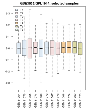 Value distribution for the yeast cell-cycle experiment GSE3635. Experiments are grouped approximately into equivalent time-points on a cell cycle.

- Define groups: the associated publication shows us that one cell-cycle takes pretty exactly 60 minutes. Create timepoints T0, T1, T2, ... T5. Then associate the 0 and 60 min. sample with "T0"; 10 and 70 minutes get grouped as "T1"; 20 and 80 minutes are T2, etc. up to T5. The final sample does not get assigned.
- Confirm that the Value distributions are unbiased by accessing the value distribution tab - overall, in such experiments, the bulk of the expression values should not change and thus means and quantiles of the expression levels should be about the same.
- Your distribution should look like the image on the right: properly grouped into six categories, and unbiased regarding absolute expression levels and trends.
- Look for differentially expressed genes: open the GEO2R tab and click on Top 250.
- Analyze the results.
- Examine the top hits. Click on a few of the gene names in the Gene.symbol column to view the expression profiles that tell you why the genes were found to be differentially expressed. What do you think? Is this what you would have expected for genes' responses to the cell-cycle? What seems to be the algorithm's notion of what "differentially expressed" means?
- Look for expected genes. Here are a few genes that are known to be differentially expressed in the cell-cycle as target genes of the MBF complex:
DSE1,DSE2,ERF3,HTA2,HTB2, andGAS3. But what about the MBD complex proteins themselves: Mbp1 and Swi6?
The notion of "differential expression" and "cell-cycle dependent expression" do not overlap completely. Significant differential expression is mathematically determined for genes that have low variance within groups and large differences between groups. This algorithm has no notion of any expectation you might have about the shape of the expression profile. All it finds are genes for which differential expression between some groups is statistically supported. The algorithm returns the top 250 of those. Consistency within groups is very important, while we intuitively might be giving more weight to conformance to our expectations of a cyclical pattern.
Let's see if we can group our time points differently to enhance the contrast between expression levels for cyclically expressed genes. Let's define only two groups: one set before and between the two cycles, one set at the peaks - and we'll omit some of the intermediate values.
- Remove all of your groups and define two groups only. Call them "A" and "B".
- Assign samples for T = 0 min, 10, 60 and 70 min. to the "A" group. Assign sets 30, 40, 90, and 100 to the "B" group.
- Recalculate the Top 250 differentially expressed genes (you might have to refresh the page to get the "Top 250" button back.) Which of the "known" MBF targets are now contained in the set? What about Mbp1 and Swi6?
- Finally: Let's compare the expression profiles for Mbp1, Swi6 and Swi4. It is not obvious that transcription factors are themselves under transcriptional control, as opposed to being expressed at a basal level and activated by phosporylation or ligand binding. In a new page, navigate to the Geo profiles page and enter
(Mbp1 OR Swi6 OR Swi4 OR Nrm1 OR Cln1 OR Clb6 OR Act1 OR Alg9) AND GSE3635(Nrm1, Cln1, and Clb6 are Mbp1 target genes. Act1 and Alg9 are beta-Actin and mannosyltransferase, these are often used as "housekeeping genes, i.e. genes with condition-independent expression levels, especially for qPCR studies - although Alg9 is also an Mbp1 target. We include them here as negative controls. CGSE3635 is the ID of the GEO data set we have just studied). You could have got similar results in the Profile graph tab of the GEO2R page. What do you find? What does this tell you? Would this information allow you to define groups that are even better suited for finding cyclically expressed genes? - Click on the profile graph for Mbp1 and print out the page. Write your name and student number on the page. With a red pen, in one sentence describe the evidence you find on that page that allows us to conclude whether or not Mbp1 is a cell-cycle gene. You'll probably want to think for a moment what this question really means, how a cell-cycle gene could be defined, and what can be considered "evidence", before you write. I will mark your response for a maximum of four marks.
Further reading and resources
| Okamura et al. (2015) COXPRESdb in 2015: coexpression database for animal species by DNA-microarray and RNAseq-based expression data with multiple quality assessment systems. Nucleic Acids Res 43:D82-6. (pmid: 25392420) |
|
[ PubMed ] [ DOI ] The COXPRESdb (http://coxpresdb.jp) provides gene coexpression relationships for animal species. Here, we report the updates of the database, mainly focusing on the following two points. For the first point, we added RNAseq-based gene coexpression data for three species (human, mouse and fly), and largely increased the number of microarray experiments to nine species. The increase of the number of expression data with multiple platforms could enhance the reliability of coexpression data. For the second point, we refined the data assessment procedures, for each coexpressed gene list and for the total performance of a platform. The assessment of coexpressed gene list now uses more reasonable P-values derived from platform-specific null distribution. These developments greatly reduced pseudo-predictions for directly associated genes, thus expanding the reliability of coexpression data to design new experiments and to discuss experimental results. |
| Barrett et al. (2013) NCBI GEO: archive for functional genomics data sets--update. Nucleic Acids Res 41:D991-5. (pmid: 23193258) |
|
[ PubMed ] [ DOI ] The Gene Expression Omnibus (GEO, http://www.ncbi.nlm.nih.gov/geo/) is an international public repository for high-throughput microarray and next-generation sequence functional genomic data sets submitted by the research community. The resource supports archiving of raw data, processed data and metadata which are indexed, cross-linked and searchable. All data are freely available for download in a variety of formats. GEO also provides several web-based tools and strategies to assist users to query, analyse and visualize data. This article reports current status and recent database developments, including the release of GEO2R, an R-based web application that helps users analyse GEO data. |
Protein-Protein Interactions
Task:
- Carefully read the lecture notes for this unit Week 11: Annotated Notes (PDF 12.2 MB).
- For a useful overview of graph-theory concepts you could additionally have a look at:
| Pavlopoulos et al. (2011) Using graph theory to analyze biological networks. BioData Min 4:10. (pmid: 21527005) |
|
[ PubMed ] [ DOI ] Understanding complex systems often requires a bottom-up analysis towards a systems biology approach. The need to investigate a system, not only as individual components but as a whole, emerges. This can be done by examining the elementary constituents individually and then how these are connected. The myriad components of a system and their interactions are best characterized as networks and they are mainly represented as graphs where thousands of nodes are connected with thousands of vertices. In this article we demonstrate approaches, models and methods from the graph theory universe and we discuss ways in which they can be used to reveal hidden properties and features of a network. This network profiling combined with knowledge extraction will help us to better understand the biological significance of the system. |
However, the concepts you need to know for this assignment should become clear from the notes.
Data Sources
Interaction databases have similar problems as sequence databases: the need for standards for abstracting biological concepts into computable objects, data integrity, search and retrieval, and the metrics of comparison. There is however an added complication: interactions are rarely all-or-none, and the high-throughput experimental methods have large false-positive and false-negative rates. This makes it necessary to define confidence scores for interactions. On top of experimental methods, there are also a variety of methods for computational interaction prediction. However, even though the "gold standard" are careful, small-scale laboratory experiments, different curated efforts on the same experimental publication usually lead to different results - with as little as 42% overlap between databases being reported.
Currently, likely the best integrated protein-protein interaction database is IntAct, at the EBI, which besides curating interactions from the literature hosts interactions from the IMEx consortium, an extensive data-sharing agreement between a number of general and specialized source databases.
Task:
- Access IntAct and enter the UniProt ID for yeast Mbp1 P39678.
- Click on the "Graph" tab to load a network graph.
- Switch "Merge edges" off to show the reported edges for this interaction individually. Which protein pair has the most interactions? Does this make sense?
But then what?
If you are like me, you would now like to be able to link expression profiles, information about known complexes, GO annotations, knock-out phenotypes etc. etc. Too bad.
Working with biological graphs in R
Task:
- Open RStudio.
- Choose File → Recent Projects → BCH441_2016.
- Pull the latest version of the project repository from GitHub.
- type init()
- Open the file BCH441_A11.R and work through the entire tutorial.
- At the end of the tutorial, you are being asked to print R code and data on a sheet of paper and bring this to class. This will be marked by me and worth maximally 4 marks. Be careful to follow the instructions exactly, especially regarding how to use your student number as a randomization seed.
- This is all that is required. There is optional material below that you may find interesting.
Optional: Data visualization and analysis
If you work a lot with interaction networks, sooner or later you will come across Cytoscape. It is more or less the standard among "professional" systems biologists. But it is not an online tool.
Task:
- Navigate to the Cytoscape homepage and inform yourself what the program does and how to install it. There are many tutorials online available. But this is software that needs to be downloaded, and installed and it definitively has a learning curve.
The state of integrated online interaction viewers these days could be improved. Have a look at this article that discusses the gap between what one would need to do, and what is offered:
| Jeanquartier et al. (2015) Integrated web visualizations for protein-protein interaction databases. BMC Bioinformatics 16:195. (pmid: 26077899) |
|
[ PubMed ] [ DOI ] BACKGROUND: Understanding living systems is crucial for curing diseases. To achieve this task we have to understand biological networks based on protein-protein interactions. Bioinformatics has come up with a great amount of databases and tools that support analysts in exploring protein-protein interactions on an integrated level for knowledge discovery. They provide predictions and correlations, indicate possibilities for future experimental research and fill the gaps to complete the picture of biochemical processes. There are numerous and huge databases of protein-protein interactions used to gain insights into answering some of the many questions of systems biology. Many computational resources integrate interaction data with additional information on molecular background. However, the vast number of diverse Bioinformatics resources poses an obstacle to the goal of understanding. We present a survey of databases that enable the visual analysis of protein networks. RESULTS: We selected M=10 out of N=53 resources supporting visualization, and we tested against the following set of criteria: interoperability, data integration, quantity of possible interactions, data visualization quality and data coverage. The study reveals differences in usability, visualization features and quality as well as the quantity of interactions. StringDB is the recommended first choice. CPDB presents a comprehensive dataset and IntAct lets the user change the network layout. A comprehensive comparison table is available via web. The supplementary table can be accessed on http://tinyurl.com/PPI-DB-Comparison-2015. CONCLUSIONS: Only some web resources featuring graph visualization can be successfully applied to interactive visual analysis of protein-protein interaction. Study results underline the necessity for further enhancements of visualization integration in biochemical analysis tools. Identified challenges are data comprehensiveness, confidence, interactive feature and visualization maturing. |
The online resource that comes out as the best is the one at the String database.
Task:
- Navigate to the String database and search for saccharomyces cerevisiae Mbp1 interactors.
- Visualize the network. Add a few proteins by clicking the (+) button a two or three times.
- Click on a node to get a synopsis of its function.
- Explore the "confidence", "evidence" and "actions" networks for the retrieved interactors.
- Not all interacting proteins are also predicted to have a functional relationship with Mbp1. Do you agree?
- Explore the clustering and layout options. Do you understand what they do?
- Explore the Views on
- Neighborhood (not relevant for our query though)
- Fusion (also not relevant for our query)
- Occurence
- Coexpression
- Experiments
- Database, and
- Textmining
Each of these are methods for predicting functional relationships. Figure out how each one contributes to evidence of a functional interaction between Mbp1 and its predicted functional partners. I find the Occurrence view a unique and intriguing tool: visualizing in which organisms groups of genes are either all absent or all present allows to quickly establish functional clusters.
In summary, String is a convincingly well built tool to explore functional relationships between proteins.
Links and resources
| Pavlopoulos et al. (2011) Using graph theory to analyze biological networks. BioData Min 4:10. (pmid: 21527005) |
|
[ PubMed ] [ DOI ] Understanding complex systems often requires a bottom-up analysis towards a systems biology approach. The need to investigate a system, not only as individual components but as a whole, emerges. This can be done by examining the elementary constituents individually and then how these are connected. The myriad components of a system and their interactions are best characterized as networks and they are mainly represented as graphs where thousands of nodes are connected with thousands of vertices. In this article we demonstrate approaches, models and methods from the graph theory universe and we discuss ways in which they can be used to reveal hidden properties and features of a network. This network profiling combined with knowledge extraction will help us to better understand the biological significance of the system. |
EC
Enzyme Commission Codes ...
GO
Introduction
| Harris (2008) Developing an ontology. Methods Mol Biol 452:111-24. (pmid: 18563371) |
|
[ PubMed ] [ DOI ] In recent years, biological ontologies have emerged as a means of representing and organizing biological concepts, enabling biologists, bioinformaticians, and others to derive meaning from large datasets.This chapter provides an overview of formal principles and practical considerations of ontology construction and application. Ontology development concepts are illustrated using examples drawn from the Gene Ontology (GO) and other OBO ontologies. |
| Hackenberg & Matthiesen (2010) Algorithms and methods for correlating experimental results with annotation databases. Methods Mol Biol 593:315-40. (pmid: 19957156) |
|
[ PubMed ] [ DOI ] An important procedure in biomedical research is the detection of genes that are differentially expressed under pathologic conditions. These genes, or at least a subset of them, are key biomarkers and are thought to be important to describe and understand the analyzed biological system (the pathology) at a molecular level. To obtain this understanding, it is indispensable to link those genes to biological knowledge stored in databases. Ontological analysis is nowadays a standard procedure to analyze large gene lists. By detecting enriched and depleted gene properties and functions, important insights on the biological system can be obtained. In this chapter, we will give a brief survey of the general layout of the methods used in an ontological analysis and of the most important tools that have been developed. |
GO
The Gene Ontology project is the most influential contributor to the definition of function in computational biology and the use of GO terms and GO annotations is ubiquitous.
|
GO: the Gene Ontology project [ link ] [ page ] Ontologies are important tools to organize and compute with non-standardized information, such as gene annotations. The Gene Ontology project (GO) constructs ontologies for gene and gene product attributes across numerous species. Three major ontologies are being developed: molecular process, biological function and cellular location. Each includes terms, their definition, and their relationships. In addition, genes and gene products are being been annotated with their GO terms and the type of evidence that underlies the annotation. A number of tools such as the AmiGO browser are available to analyse relationships, construct ontologies and curate annotations. Data can be freely downloaded in formats that are convenient for computation. |  |
| du Plessis et al. (2011) The what, where, how and why of gene ontology--a primer for bioinformaticians. Brief Bioinformatics 12:723-35. (pmid: 21330331) |
|
[ PubMed ] [ DOI ] With high-throughput technologies providing vast amounts of data, it has become more important to provide systematic, quality annotations. The Gene Ontology (GO) project is the largest resource for cataloguing gene function. Nonetheless, its use is not yet ubiquitous and is still fraught with pitfalls. In this review, we provide a short primer to the GO for bioinformaticians. We summarize important aspects of the structure of the ontology, describe sources and types of functional annotations, survey measures of GO annotation similarity, review typical uses of GO and discuss other important considerations pertaining to the use of GO in bioinformatics applications. |
The GO actually comprises three separate ontologies:
- Molecular function
- ...
- Biological Process
- ...
- Cellular component
- ...
GO terms
GO terms comprise the core of the information in the ontology: a carefully crafted definition of a term in any of GO's separate ontologies.
GO relationships
The nature of the relationships is as much a part of the ontology as the terms themselves. GO uses three categories of relationships:
- is a
- part of
- regulates
GO annotations
The GO terms are conceptual in nature, and while they represent our interpretation of biological phenomena, they do not intrinsically represent biological objects, such a specific genes or proteins. In order to link molecules with these concepts, the ontology is used to annotate genes. The annotation project is referred to as GOA.
| Dimmer et al. (2007) Methods for gene ontology annotation. Methods Mol Biol 406:495-520. (pmid: 18287709) |
|
[ PubMed ] [ DOI ] The Gene Ontology (GO) is an established dynamic and structured vocabulary that has been successfully used in gene and protein annotation. Designed by biologists to improve data integration, GO attempts to replace the multiple nomenclatures used by specialised and large biological knowledgebases. This chapter describes the methods used by groups to create new GO annotations and how users can apply publicly available GO annotations to enhance their datasets. |
GO evidence codes
Annotations can be made according to literature data or computational inference and it is important to note how an annotation has been justified by the curator to evaluate the level of trust we should have in the annotation. GO uses evidence codes to make this process transparent. When computing with the ontology, we may want to filter (exclude) particular terms in order to avoid tautologies: for example if we were to infer functional relationships between homologous genes, we should exclude annotations that have been based on the same inference or similar, and compute only with the actual experimental data.
The following evidence codes are in current use; if you want to exclude inferred anotations you would restrict the codes you use to the ones shown in bold: EXP, IDA, IPI, IMP, IEP, and perhaps IGI, although the interpretation of genetic interactions can require assumptions.
- Automatically-assigned Evidence Codes
- IEA: Inferred from Electronic Annotation
- Curator-assigned Evidence Codes
- Experimental Evidence Codes
- EXP: Inferred from Experiment
- IDA: Inferred from Direct Assay
- IPI: Inferred from Physical Interaction
- IMP: Inferred from Mutant Phenotype
- IGI: Inferred from Genetic Interaction
- IEP: Inferred from Expression Pattern
- Computational Analysis Evidence Codes
- ISS: Inferred from Sequence or Structural Similarity
- ISO: Inferred from Sequence Orthology
- ISA: Inferred from Sequence Alignment
- ISM: Inferred from Sequence Model
- IGC: Inferred from Genomic Context
- IBA: Inferred from Biological aspect of Ancestor
- IBD: Inferred from Biological aspect of Descendant
- IKR: Inferred from Key Residues
- IRD: Inferred from Rapid Divergence
- RCA: inferred from Reviewed Computational Analysis
- Author Statement Evidence Codes
- TAS: Traceable Author Statement
- NAS: Non-traceable Author Statement
- Curator Statement Evidence Codes
- IC: Inferred by Curator
- ND: No biological Data available
For further details, see the Guide to GO Evidence Codes and the GO Evidence Code Decision Tree.
GO tools
For many projects, the simplest approach will be to download the GO ontology itself. It is a well constructed, easily parseable file that is well suited for computation. For details, see Computing with GO on this wiki.
AmiGO
practical work with GO: at first via the AmiGO browser AmiGO is a GO browser developed by the Gene Ontology consortium and hosted on their website.
AmiGO - Gene products
Task:
- Navigate to the GO homepage.
- Enter
SOX2into the search box to initiate a search for the human SOX2 transcription factor (WP, HUGO) (as gene or protein name). - There are a number of hits in various organisms: sulfhydryl oxidases and (sex determining region Y)-box genes. Check to see the various ways by which you could filter and restrict the results.
- Select Homo sapiens as the species filter and set the filter. Note that this still does not give you a unique hit, but ...
- ... you can identify the Transcription factor SOX-2 and follow its gene product information link. Study the information on that page.
- Later, we will need Entrez Gene IDs. The GOA information page provides these as GeneID in the External references section. Note it down. With the same approach, find and record the Gene IDs (a) of the functionally related Oct4 (POU5F1) protein, (b) the human cell-cycle transcription factor E2F1, (c) the human bone morphogenetic protein-4 transforming growth factor BMP4, (d) the human UDP glucuronosyltransferase 1 family protein 1, an enzyme that is differentially expressed in some cancers, UGT1A1, and (d) as a positive control, SOX2's interaction partner NANOG, which we would expect to be annotated as functionally similar to both Oct4 and SOX2.
AmiGO - Associations
GO annotations for a protein are called associations.
Task:
- Open the associations information page for the human SOX2 protein via the link in the right column in a separate tab. Study the information on that page.
- Note that you can filter the associations by ontology and evidence code. You have read about the three GO ontologies in your previous assignment, but you should also be familiar with the evidence codes. Click on any of the evidence links to access the Evidence code definition page and study the definitions of the codes. Make sure you understand which codes point to experimental observation, and which codes denote computational inference, or say that the evidence is someone's opinion (TAS, IC etc.). Note: it is good practice - but regrettably not universally implemented standard - to clearly document database semantics and keep definitions associated with database entries easily accessible, as GO is doing here. You won't find this everywhere, but as a user please feel encouraged to complain to the database providers if you come across a database where the semantics are not clear. Seriously: opaque semantics make database annotations useless.
- There are many associations (around 60) and a good way to select which ones to pursue is to follow the most specific ones. Set
IDAas a filter and among the returned terms selectGO:0035019– somatic stem cell maintenance in the Biological Process ontology. Follow that link. - Study the information available on that page and through the tabs on the page, especially the graph view.
- In the Inferred Tree View tab, find the genes annotated to this go term for homo sapiens. There should be about 55. Click on the number behind the term. The resulting page will give you all human proteins that have been annotated with this particular term. Note that the great majority of these is via the
IEAevidence code.
Semantic similarity
A good, recent overview of ontology based functional annotation is found in the following article. This is not a formal reading assignment, but do familiarize yourself with section 3: Derivation of Semantic Similarity between Terms in an Ontology as an introduction to the code-based annotations below.
| Gan et al. (2013) From ontology to semantic similarity: calculation of ontology-based semantic similarity. ScientificWorldJournal 2013:793091. (pmid: 23533360) |
|
[ PubMed ] [ DOI ] Advances in high-throughput experimental techniques in the past decade have enabled the explosive increase of omics data, while effective organization, interpretation, and exchange of these data require standard and controlled vocabularies in the domain of biological and biomedical studies. Ontologies, as abstract description systems for domain-specific knowledge composition, hence receive more and more attention in computational biology and bioinformatics. Particularly, many applications relying on domain ontologies require quantitative measures of relationships between terms in the ontologies, making it indispensable to develop computational methods for the derivation of ontology-based semantic similarity between terms. Nevertheless, with a variety of methods available, how to choose a suitable method for a specific application becomes a problem. With this understanding, we review a majority of existing methods that rely on ontologies to calculate semantic similarity between terms. We classify existing methods into five categories: methods based on semantic distance, methods based on information content, methods based on properties of terms, methods based on ontology hierarchy, and hybrid methods. We summarize characteristics of each category, with emphasis on basic notions, advantages and disadvantages of these methods. Further, we extend our review to software tools implementing these methods and applications using these methods. |
Practical work with GO: bioconductor.
The bioconductor project hosts the GOSemSim package for semantic similarity.
Task:
- Work through the following R-code. If you have problems, discuss them on the mailing list. Don't go through the code mechanically but make sure you are clear about what it does.
# GOsemanticSimilarity.R
# GO semantic similarity example
# B. Steipe for BCB420, January 2014

setwd("~/your-R-project-directory")

# GOSemSim is an R-package in the bioconductor project. It is not installed via
# the usual install.packages() comand (via CRAN) but via an installation script
# that is run from the bioconductor Website.

source("http://bioconductor.org/biocLite.R")
biocLite("GOSemSim")

library(GOSemSim)

# This loads the library and starts the Bioconductor environment.
# You can get an overview of functions by executing ...
browseVignettes()
# ... which will open a listing in your Web browser. Open the
# introduction to GOSemSim PDF. As the introduction suggests,
# now is a good time to execute ...
help(GOSemSim)

# The simplest function is to measure the semantic similarity of two GO
# terms. For example, SOX2 was annotated with GO:0035019 (somatic stem cell
# maintenance), QSOX2 was annotated with GO:0045454 (cell redox homeostasis),
# and Oct4 (POU5F1) with GO:0009786 (regulation of asymmetric cell division),
# among other associations. Lets calculate these similarities.
goSim("GO:0035019", "GO:0009786", ont="BP", measure="Wang")
goSim("GO:0035019", "GO:0045454", ont="BP", measure="Wang")

# Fair enough. Two numbers. Clearly we would appreciate an idea of the values
# that high similarity and low similarity can take. But in any case -
# we are really less interested in the similarity of GO terms - these
# are a function of how the Ontology was constructed. We are more
# interested in the functional similarity of our genes, and these
# have a number of GO terms associated with them.

# GOSemSim provides the functions ...
?geneSim()
?mgeneSim()
# ... to compute these values. Refer to the vignette for details, in
# particular, consider how multiple GO terms are combined, and how to
# keep/drop evidence codes.
# Here is a pairwise similarity example: the gene IDs are the ones you
# have recorded previously. Note that this will download a package
# of GO annotations - you might not want to do this on a low-bandwidth
# connection.
geneSim("6657", "5460", ont = "BP", measure="Wang", combine = "BMA")
# Another number. And the list of GO terms that were considered.

# Your task: use the mgeneSim() function to calculate the similarities
# between all six proteins for which you have recorded the GeneIDs
# previously (SOX2, POU5F1, E2F1, BMP4, UGT1A1 and NANOG) in the
# biological process ontology.

# This will run for some time. On my machine, half an hour or so.

# Do the results correspond to your expectations?
GO reading and resources
- General
| Sauro & Bergmann (2008) Standards and ontologies in computational systems biology. Essays Biochem 45:211-22. (pmid: 18793134) |
|
[ PubMed ] [ DOI ] With the growing importance of computational models in systems biology there has been much interest in recent years to develop standard model interchange languages that permit biologists to easily exchange models between different software tools. In the present chapter two chief model exchange standards, SBML (Systems Biology Markup Language) and CellML are described. In addition, other related features including visual layout initiatives, ontologies and best practices for model annotation are discussed. Software tools such as developer libraries and basic editing tools are also introduced, together with a discussion on the future of modelling languages and visualization tools in systems biology. |
- Phenotype etc. Ontologies
See also:
| Köhler et al. (2014) The Human Phenotype Ontology project: linking molecular biology and disease through phenotype data. Nucleic Acids Res 42:D966-74. (pmid: 24217912) |
|
[ PubMed ] [ DOI ] The Human Phenotype Ontology (HPO) project, available at http://www.human-phenotype-ontology.org, provides a structured, comprehensive and well-defined set of 10,088 classes (terms) describing human phenotypic abnormalities and 13,326 subclass relations between the HPO classes. In addition we have developed logical definitions for 46% of all HPO classes using terms from ontologies for anatomy, cell types, function, embryology, pathology and other domains. This allows interoperability with several resources, especially those containing phenotype information on model organisms such as mouse and zebrafish. Here we describe the updated HPO database, which provides annotations of 7,278 human hereditary syndromes listed in OMIM, Orphanet and DECIPHER to classes of the HPO. Various meta-attributes such as frequency, references and negations are associated with each annotation. Several large-scale projects worldwide utilize the HPO for describing phenotype information in their datasets. We have therefore generated equivalence mappings to other phenotype vocabularies such as LDDB, Orphanet, MedDRA, UMLS and phenoDB, allowing integration of existing datasets and interoperability with multiple biomedical resources. We have created various ways to access the HPO database content using flat files, a MySQL database, and Web-based tools. All data and documentation on the HPO project can be found online. |
| Schriml et al. (2012) Disease Ontology: a backbone for disease semantic integration. Nucleic Acids Res 40:D940-6. (pmid: 22080554) |
|
[ PubMed ] [ DOI ] The Disease Ontology (DO) database (http://disease-ontology.org) represents a comprehensive knowledge base of 8043 inherited, developmental and acquired human diseases (DO version 3, revision 2510). The DO web browser has been designed for speed, efficiency and robustness through the use of a graph database. Full-text contextual searching functionality using Lucene allows the querying of name, synonym, definition, DOID and cross-reference (xrefs) with complex Boolean search strings. The DO semantically integrates disease and medical vocabularies through extensive cross mapping and integration of MeSH, ICD, NCI's thesaurus, SNOMED CT and OMIM disease-specific terms and identifiers. The DO is utilized for disease annotation by major biomedical databases (e.g. Array Express, NIF, IEDB), as a standard representation of human disease in biomedical ontologies (e.g. IDO, Cell line ontology, NIFSTD ontology, Experimental Factor Ontology, Influenza Ontology), and as an ontological cross mappings resource between DO, MeSH and OMIM (e.g. GeneWiki). The DO project (http://diseaseontology.sf.net) has been incorporated into open source tools (e.g. Gene Answers, FunDO) to connect gene and disease biomedical data through the lens of human disease. The next iteration of the DO web browser will integrate DO's extended relations and logical definition representation along with these biomedical resource cross-mappings. |
| Evelo et al. (2011) Answering biological questions: querying a systems biology database for nutrigenomics. Genes Nutr 6:81-7. (pmid: 21437033) |
|
[ PubMed ] [ DOI ] The requirement of systems biology for connecting different levels of biological research leads directly to a need for integrating vast amounts of diverse information in general and of omics data in particular. The nutritional phenotype database addresses this challenge for nutrigenomics. A particularly urgent objective in coping with the data avalanche is making biologically meaningful information accessible to the researcher. This contribution describes how we intend to meet this objective with the nutritional phenotype database. We outline relevant parts of the system architecture, describe the kinds of data managed by it, and show how the system can support retrieval of biologically meaningful information by means of ontologies, full-text queries, and structured queries. Our contribution points out critical points, describes several technical hurdles. It demonstrates how pathway analysis can improve queries and comparisons for nutrition studies. Finally, three directions for future research are given. |
| Oti et al. (2009) The biological coherence of human phenome databases. Am J Hum Genet 85:801-8. (pmid: 20004759) |
|
[ PubMed ] [ DOI ] Disease networks are increasingly explored as a complement to networks centered around interactions between genes and proteins. The quality of disease networks is heavily dependent on the amount and quality of phenotype information in phenotype databases of human genetic diseases. We explored which aspects of phenotype database architecture and content best reflect the underlying biology of disease. We used the OMIM-based HPO, Orphanet, and POSSUM phenotype databases for this purpose and devised a biological coherence score based on the sharing of gene ontology annotation to investigate the degree to which phenotype similarity in these databases reflects related pathobiology. Our analyses support the notion that a fine-grained phenotype ontology enhances the accuracy of phenome representation. In addition, we find that the OMIM database that is most used by the human genetics community is heavily underannotated. We show that this problem can easily be overcome by simply adding data available in the POSSUM database to improve OMIM phenotype representations in the HPO. Also, we find that the use of feature frequency estimates--currently implemented only in the Orphanet database--significantly improves the quality of the phenome representation. Our data suggest that there is much to be gained by improving human phenome databases and that some of the measures needed to achieve this are relatively easy to implement. More generally, we propose that curation and more systematic annotation of human phenome databases can greatly improve the power of the phenotype for genetic disease analysis. |
| Groth et al. (2007) PhenomicDB: a new cross-species genotype/phenotype resource. Nucleic Acids Res 35:D696-9. (pmid: 16982638) |
|
[ PubMed ] [ DOI ] Phenotypes are an important subject of biomedical research for which many repositories have already been created. Most of these databases are either dedicated to a single species or to a single disease of interest. With the advent of technologies to generate phenotypes in a high-throughput manner, not only is the volume of phenotype data growing fast but also the need to organize these data in more useful ways. We have created PhenomicDB (freely available at http://www.phenomicdb.de), a multi-species genotype/phenotype database, which shows phenotypes associated with their corresponding genes and grouped by gene orthologies across a variety of species. We have enhanced PhenomicDB recently by additionally incorporating quantitative and descriptive RNA interference (RNAi) screening data, by enabling the usage of phenotype ontology terms and by providing information on assays and cell lines. We envision that integration of classical phenotypes with high-throughput data will bring new momentum and insights to our understanding. Modern analysis tools under development may help exploiting this wealth of information to transform it into knowledge and, eventually, into novel therapeutic approaches. |
- Semantic similarity
| Wu et al. (2013) Improving the measurement of semantic similarity between gene ontology terms and gene products: insights from an edge- and IC-based hybrid method. PLoS ONE 8:e66745. (pmid: 23741529) |
|
[ PubMed ] [ DOI ] BACKGROUND: Explicit comparisons based on the semantic similarity of Gene Ontology terms provide a quantitative way to measure the functional similarity between gene products and are widely applied in large-scale genomic research via integration with other models. Previously, we presented an edge-based method, Relative Specificity Similarity (RSS), which takes the global position of relevant terms into account. However, edge-based semantic similarity metrics are sensitive to the intrinsic structure of GO and simply consider terms at the same level in the ontology to be equally specific nodes, revealing the weaknesses that could be complemented using information content (IC). RESULTS AND CONCLUSIONS: Here, we used the IC-based nodes to improve RSS and proposed a new method, Hybrid Relative Specificity Similarity (HRSS). HRSS outperformed other methods in distinguishing true protein-protein interactions from false. HRSS values were divided into four different levels of confidence for protein interactions. In addition, HRSS was statistically the best at obtaining the highest average functional similarity among human-mouse orthologs. Both HRSS and the groupwise measure, simGIC, are superior in correlation with sequence and Pfam similarities. Because different measures are best suited for different circumstances, we compared two pairwise strategies, the maximum and the best-match average, in the evaluation. The former was more effective at inferring physical protein-protein interactions, and the latter at estimating the functional conservation of orthologs and analyzing the CESSM datasets. In conclusion, HRSS can be applied to different biological problems by quantifying the functional similarity between gene products. The algorithm HRSS was implemented in the C programming language, which is freely available from http://cmb.bnu.edu.cn/hrss. |
| Gan et al. (2013) From ontology to semantic similarity: calculation of ontology-based semantic similarity. ScientificWorldJournal 2013:793091. (pmid: 23533360) |
|
[ PubMed ] [ DOI ] Advances in high-throughput experimental techniques in the past decade have enabled the explosive increase of omics data, while effective organization, interpretation, and exchange of these data require standard and controlled vocabularies in the domain of biological and biomedical studies. Ontologies, as abstract description systems for domain-specific knowledge composition, hence receive more and more attention in computational biology and bioinformatics. Particularly, many applications relying on domain ontologies require quantitative measures of relationships between terms in the ontologies, making it indispensable to develop computational methods for the derivation of ontology-based semantic similarity between terms. Nevertheless, with a variety of methods available, how to choose a suitable method for a specific application becomes a problem. With this understanding, we review a majority of existing methods that rely on ontologies to calculate semantic similarity between terms. We classify existing methods into five categories: methods based on semantic distance, methods based on information content, methods based on properties of terms, methods based on ontology hierarchy, and hybrid methods. We summarize characteristics of each category, with emphasis on basic notions, advantages and disadvantages of these methods. Further, we extend our review to software tools implementing these methods and applications using these methods. |
| Alvarez & Yan (2011) A graph-based semantic similarity measure for the gene ontology. J Bioinform Comput Biol 9:681-95. (pmid: 22084008) |
|
[ PubMed ] [ DOI ] Existing methods for calculating semantic similarities between pairs of Gene Ontology (GO) terms and gene products often rely on external databases like Gene Ontology Annotation (GOA) that annotate gene products using the GO terms. This dependency leads to some limitations in real applications. Here, we present a semantic similarity algorithm (SSA), that relies exclusively on the GO. When calculating the semantic similarity between a pair of input GO terms, SSA takes into account the shortest path between them, the depth of their nearest common ancestor, and a novel similarity score calculated between the definitions of the involved GO terms. In our work, we use SSA to calculate semantic similarities between pairs of proteins by combining pairwise semantic similarities between the GO terms that annotate the involved proteins. The reliability of SSA was evaluated by comparing the resulting semantic similarities between proteins with the functional similarities between proteins derived from expert annotations or sequence similarity. Comparisons with existing state-of-the-art methods showed that SSA is highly competitive with the other methods. SSA provides a reliable measure for semantics similarity independent of external databases of functional-annotation observations. |
| Jain & Bader (2010) An improved method for scoring protein-protein interactions using semantic similarity within the gene ontology. BMC Bioinformatics 11:562. (pmid: 21078182) |
|
[ PubMed ] [ DOI ] BACKGROUND: Semantic similarity measures are useful to assess the physiological relevance of protein-protein interactions (PPIs). They quantify similarity between proteins based on their function using annotation systems like the Gene Ontology (GO). Proteins that interact in the cell are likely to be in similar locations or involved in similar biological processes compared to proteins that do not interact. Thus the more semantically similar the gene function annotations are among the interacting proteins, more likely the interaction is physiologically relevant. However, most semantic similarity measures used for PPI confidence assessment do not consider the unequal depth of term hierarchies in different classes of cellular location, molecular function, and biological process ontologies of GO and thus may over-or under-estimate similarity. RESULTS: We describe an improved algorithm, Topological Clustering Semantic Similarity (TCSS), to compute semantic similarity between GO terms annotated to proteins in interaction datasets. Our algorithm, considers unequal depth of biological knowledge representation in different branches of the GO graph. The central idea is to divide the GO graph into sub-graphs and score PPIs higher if participating proteins belong to the same sub-graph as compared to if they belong to different sub-graphs. CONCLUSIONS: The TCSS algorithm performs better than other semantic similarity measurement techniques that we evaluated in terms of their performance on distinguishing true from false protein interactions, and correlation with gene expression and protein families. We show an average improvement of 4.6 times the F1 score over Resnik, the next best method, on our Saccharomyces cerevisiae PPI dataset and 2 times on our Homo sapiens PPI dataset using cellular component, biological process and molecular function GO annotations. |
| Yu et al. (2010) GOSemSim: an R package for measuring semantic similarity among GO terms and gene products. Bioinformatics 26:976-8. (pmid: 20179076) |
|
[ PubMed ] [ DOI ] SUMMARY: The semantic comparisons of Gene Ontology (GO) annotations provide quantitative ways to compute similarities between genes and gene groups, and have became important basis for many bioinformatics analysis approaches. GOSemSim is an R package for semantic similarity computation among GO terms, sets of GO terms, gene products and gene clusters. Four information content (IC)- and a graph-based methods are implemented in the GOSemSim package, multiple species including human, rat, mouse, fly and yeast are also supported. The functions provided by the GOSemSim offer flexibility for applications, and can be easily integrated into high-throughput analysis pipelines. AVAILABILITY: GOSemSim is released under the GNU General Public License within Bioconductor project, and freely available at http://bioconductor.org/packages/2.6/bioc/html/GOSemSim.html. |
- GO
| Gene Ontology Consortium (2012) The Gene Ontology: enhancements for 2011. Nucleic Acids Res 40:D559-64. (pmid: 22102568) |
|
[ PubMed ] [ DOI ] The Gene Ontology (GO) (http://www.geneontology.org) is a community bioinformatics resource that represents gene product function through the use of structured, controlled vocabularies. The number of GO annotations of gene products has increased due to curation efforts among GO Consortium (GOC) groups, including focused literature-based annotation and ortholog-based functional inference. The GO ontologies continue to expand and improve as a result of targeted ontology development, including the introduction of computable logical definitions and development of new tools for the streamlined addition of terms to the ontology. The GOC continues to support its user community through the use of e-mail lists, social media and web-based resources. |
| Bastos et al. (2011) Application of gene ontology to gene identification. Methods Mol Biol 760:141-57. (pmid: 21779995) |
|
[ PubMed ] [ DOI ] Candidate gene identification deals with associating genes to underlying biological phenomena, such as diseases and specific disorders. It has been shown that classes of diseases with similar phenotypes are caused by functionally related genes. Currently, a fair amount of knowledge about the functional characterization can be found across several public databases; however, functional descriptors can be ambiguous, domain specific, and context dependent. In order to cope with these issues, the Gene Ontology (GO) project developed a bio-ontology of broad scope and wide applicability. Thus, the structured and controlled vocabulary of terms provided by the GO project describing the biological roles of gene products can be very helpful in candidate gene identification approaches. The method presented here uses GO annotation data in order to identify the most meaningful functional aspects occurring in a given set of related gene products. The method measures this meaningfulness by calculating an e-value based on the frequency of annotation of each GO term in the set of gene products versus the total frequency of annotation. Then after selecting a GO term related to the underlying biological phenomena being studied, the method uses semantic similarity to rank the given gene products that are annotated to the term. This enables the user to further narrow down the list of gene products and identify those that are more likely of interest. |
| Gene Ontology Consortium (2010) The Gene Ontology in 2010: extensions and refinements. Nucleic Acids Res 38:D331-5. (pmid: 19920128) |
|
[ PubMed ] [ DOI ] The Gene Ontology (GO) Consortium (http://www.geneontology.org) (GOC) continues to develop, maintain and use a set of structured, controlled vocabularies for the annotation of genes, gene products and sequences. The GO ontologies are expanding both in content and in structure. Several new relationship types have been introduced and used, along with existing relationships, to create links between and within the GO domains. These improve the representation of biology, facilitate querying, and allow GO developers to systematically check for and correct inconsistencies within the GO. Gene product annotation using GO continues to increase both in the number of total annotations and in species coverage. GO tools, such as OBO-Edit, an ontology-editing tool, and AmiGO, the GOC ontology browser, have seen major improvements in functionality, speed and ease of use. |
Carol Goble on the tension between purists and pragmatists in life-science ontology construction. Plenary talk at SOFG2...
| Goble & Wroe (2004) The Montagues and the Capulets. Comp Funct Genomics 5:623-32. (pmid: 18629186) |
|
[ PubMed ] [ DOI ] Two households, both alike in dignity, In fair Genomics, where we lay our scene, (One, comforted by its logic's rigour, Claims ontology for the realm of pure, The other, with blessed scientist's vigour, Acts hastily on models that endure), From ancient grudge break to new mutiny, When 'being' drives a fly-man to blaspheme. From forth the fatal loins of these two foes, Researchers to unlock the book of life; Whole misadventured piteous overthrows, Can with their work bury their clans' strife. The fruitful passage of their GO-mark'd love, And the continuance of their studies sage, Which, united, yield ontologies undreamed-of, Is now the hour's traffic of our stage; The which if you with patient ears attend, What here shall miss, our toil shall strive to mend. |
| Gajiwala & Burley (2000) Winged helix proteins. Curr Opin Struct Biol 10:110-6. (pmid: 10679470) |
|
[ PubMed ] [ DOI ] The winged helix proteins constitute a subfamily within the large ensemble of helix-turn-helix proteins. Since the discovery of the winged helix/fork head motif in 1993, a large number of topologically related proteins with diverse biological functions have been characterized by X-ray crystallography and solution NMR spectroscopy. Recently, a winged helix transcription factor (RFX1) was shown to bind DNA using unprecedented interactions between one of its eponymous wings and the major groove. This surprising observation suggests that the winged helix proteins can be subdivided into at least two classes with radically different modes of DNA recognition. |
| Aravind et al. (2005) The many faces of the helix-turn-helix domain: transcription regulation and beyond. FEMS Microbiol Rev 29:231-62. (pmid: 15808743) |
|
[ PubMed ] [ DOI ] The helix-turn-helix (HTH) domain is a common denominator in basal and specific transcription factors from the three super-kingdoms of life. At its core, the domain comprises of an open tri-helical bundle, which typically binds DNA with the 3rd helix. Drawing on the wealth of data that has accumulated over two decades since the discovery of the domain, we present an overview of the natural history of the HTH domain from the viewpoint of structural analysis and comparative genomics. In structural terms, the HTH domains have developed several elaborations on the basic 3-helical core, such as the tetra-helical bundle, the winged-helix and the ribbon-helix-helix type configurations. In functional terms, the HTH domains are present in the most prevalent transcription factors of all prokaryotic genomes and some eukaryotic genomes. They have been recruited to a wide range of functions beyond transcription regulation, which include DNA repair and replication, RNA metabolism and protein-protein interactions in diverse signaling contexts. Beyond their basic role in mediating macromolecular interactions, the HTH domains have also been incorporated into the catalytic domains of diverse enzymes. We discuss the general domain architectural themes that have arisen amongst the HTH domains as a result of their recruitment to these diverse functions. We present a natural classification, higher-order relationships and phyletic pattern analysis of all the major families of HTH domains. This reconstruction suggests that there were at least 6-11 different HTH domains in the last universal common ancestor of all life forms, which covered much of the structural diversity and part of the functional versatility of the extant representatives of this domain. In prokaryotes the total number of HTH domains per genome shows a strong power-equation type scaling with the gene number per genome. However, the HTH domains in two-component signaling pathways show a linear scaling with gene number, in contrast to the non-linear scaling of HTH domains in single-component systems and sigma factors. These observations point to distinct evolutionary forces in the emergence of different signaling systems with HTH transcription factors. The archaea and bacteria share a number of ancient families of specific HTH transcription factors. However, they do not share any orthologous HTH proteins in the basal transcription apparatus. This differential relationship of their basal and specific transcriptional machinery poses an apparent conundrum regarding the origins of their transcription apparatus. |
Footnotes and references
- ↑ Strictly speaking, splicing is an eukaryotic achievement, however there are examples of splicing in prokaryotes as well.
- ↑
(2015) The noncoding explosion. Nat Struct Mol Biol 22:1. (pmid: 25565024) Jarvis & Robertson (2011) The noncoding universe. BMC Biol 9:52. (pmid: 21798102)
Ask, if things don't work for you!
- If anything about this page is not clear to you, please ask on the mailing list. You can be certain that others will have had similar problems. Success comes from joining the conversation.
- Do consider how to ask your questions so that a meaningful answer is possible:
- Review Netiquette for the course mailing list.
- Read How to create a Minimal, Complete, and Verifiable example on stackoverflow and ...
- How to make a great R reproducible example.
| Data | Sequence | Structure | Phylogeny | Function |