Bioinformatics Introduction Data
Data
| Data | Sequence | Structure | Phylogeny | Function |
Contents
The Data Unit
This Unit is part of a brief introduction to bioinformatics. The material is more or less interleaved with the Data.R Project File which is part of the RStudio project associated with this material. Refer to the course/workshop page for installation instructions.
This Unit introduces a scenario of inquiry into cell cycle control proteins that we will loosely refer to in our explorations, explores online sources for sequence and annotation data, discusses various ways to store data in tables, spreadsheets and databases and introduces you to creating a relational data model, which is expanded on in the associated R scripts.
Scenario
In this series of introductory units we will tie contents together by exploring the system that regulates the G1/S transition in fungi, simply because it is a reasonably well analyzed regulatory system. We will focus on the Mbp1 protein in selected species from the kingdom of fungi, whose genome has been completely sequenced; our quest is thus also an exercise in model-organism reasoning: the transfer of knowledge from one, well-studied organism to others. It's reasonable to hypothesize that such central control machinery is conserved in most if not all fungi. While we know a fair bit about Mbp1, we don't know very much at all about the related genes in other organisms: whether they exist, whether they have similar functional features and whether they might contribute to the G1/S checkpoint system in a similar way.
Mbp1 is a transcription factor that plays an important role in the regulation of the cell cycle. The genetic regulation of budding- and fission yeast cell-cycles has been lucidly described in a highly recommended review by McInerny (2011)[1] (see also the short, recent introduction to cell-cycle regulated transcription by McInerny (2016)[2]). Mbp1 is a key component of the MBF complex (Mbp1/Swi6) in yeast. This complex regulates gene expression at the crucial G1/S-phase transition of the mitotic cell cycle and has been shown to bind to the regulatory regions of more than a hundred target genes. It is therefore a DNA binding protein that acts as a control switch for a key cellular process, it is highly conserved across species, and it functional analogues play a role in human disease.
Baker's yeast, Saccharomyces cerevisiae, is one of the most important model organisms, a eukaryote that has been studied genetically and biochemically in great detail for many decades. It is of very great economic importance, used in making bread and beer and other staples, and it is easily manipulated with high-throughput experimental methods.
The much less well defined organism we will explore is Spizellomyces punctatus, a recently sequenced, archaic, soil dwelling fungus.
Online Data Sources
SGD - a Yeast Model Organism Database
Yeast happens to have a very well maintained model organism database - a Web resource dedicated to Saccharomyces cerevisiae. Where such resources are available, they are very useful for the community. For the general case however, we need to work with one of the large, general data providers - the NCBI and the EBI. But in order to get a sense of the type of data that is available, let's visit the SGD database first.
Task:
Access the information page on Mbp1 at the Saccharomyces Genome Database.
- Browse through the Summary page and note the available information: you should see:
- information about the gene and the protein;
- Information about it's roles in the cell curated at the Gene Ontology database;
- Information about knock-out phenotypes; (Amazing. Would you have imagined that one of the key regulators of the cell-cycle is is a non-essential gene?)
- Information about protein-protein interactions;
- Regulation and expression;
- A curators' summary of our understanding of the protein. Mandatory reading.
- And key references.
- Access the Protein tab and note the much more detailed information.
- Domains and their classification;
- Sequence;
- Shared domains;
- and much more...
You will notice that some of this information relates to the molecule itself, and some of it relates to its relationship with other molecules. Some of it is stored at SGD, and some of it is cross-referenced from other databases. And we have textual data, numeric data, and images.
How would you store such data to use it in your project? We will define and construct a data model later in this unit.
If we would be working on yeast, most data we need is right here: curated, kept current and consistent, referenced to the literature and ready to use. But if you are working on a different species, you'll need to integrate data yourself, from data sources such as the NCBI, or UniProt. The upside is that most of the information like this is available for many, many species. The downside is that it's a challenge to map it from yeast to your target organism, and to integrate it.
NCBI databases
The NCBI (National Center for Biotechnology Information) is the largest international provider of data for genomics and molecular biology. With its annual budget of several hundred million dollars, it organizes a challenging program of data management at the largest scale, it makes its data freely and openly available over the Internet, worldwide, and it runs significant in-house research projects.
Let us explore some of the offerings of the NCBI that can contribute to our objective of studying a particular gene in an organism of interest.
Entrez
Task:
- Access the NCBI website at http://www.ncbi.nlm.nih.gov/ [3]
- In the search bar, enter
mbp1and click Search. - On the resulting page, look for the Protein section and click on the link. What do you find?
The result page of your search in "All Databases" is the "Global Query Result Page" of the Entrez system. If you follow the "Protein" link, you get taken to the more than 530 sequences in the NCBI Protein database that contain the keyword "mbp1". But when you look more closely at the results, you see that the result is quite non-specific: searching by keyword retrieves a multiubiquitin chain binding protein in Arabidopsis, bacterial mannose binding proteins, a Saccharomyces protein (perhaps one that we are actually interested in), maltose binding proteins, myelin basic proteins - and much more. There must be a more specific way to search, and indeed there is. Time to read up on the Entrez system.
Task:
- Navigate to the Entrez Help Page and read about the Entrez system, especially about:
- Boolean operators,
- wildcards,
- limits, and
- filters.
- You should minimally understand:
- How to search by keyword;
- How to search by gene or protein name;
- How to restrict a search to a particular organism.
Don't skip this part, you should know the more common options and how to find the others. It would be great to have a synopsis of the most important fields for reference, wouldn't it? Some of your colleagues have collated information on the Student Wiki (A synopsis of Entrez codes). Further contributors and editors welcome!
Keyword and organism searches are pretty universal, but apart from that, each NCBI database has its own set of specific fields. You can access the keywords via the Advanced Search interface of any of the database pages.
Protein Sequence
Task:
With this knowledge we can restrict the search to proteins called "Mbp1" that occur in Baker's Yeast. Return to the Global Search page and in the search field, type:
Mbp1[protein name] AND
 "Saccharomyces cerevisiae"[organism]
This finds two proteins. Follow the link to the result CAA98618.1—a data record in Genbank Flat File (GFF) format[4]. The database identifier CAA98618.1 tells you that this is a record in the GenPept database. There are actually several, identical versions of this sequence in the NCBI's holdings. A link to "Identical Proteins" near the top of the record shows you what these are:
Some of the sequences represent duplicate entries of the same gene (Mbp1) in the same strain (S288c) of the same species (S. cerevisiae). In particular:
- there are seven records for which the source is the INSDC, these are archival entries, submitted by independent yeast genome research projects;
- there two entries in the RefSeq database linking to the same protein:
NP_010227.1. One is derived from genome sequence, the other from mRNA. This RefSeq entry is the preferred version of the sequence for us to work with. RefSeq is a curated, non-redundant database which solves a number of problems of archival databases. You can recognize RefSeq identifiers – they always look like NP_12345.1, NM_12345.1, XP_12345.1, NC_12345.1 etc. This reflects whether the sequence is protein, mRNA or genomic, and inferred or obtained through experimental evidence. The RefSeq IDNP_010227.1actually appears twice, once linked to its genomic sequence, and once to its mRNA.
- there is a SwissProt sequence
P39678.1[5]. This link is kind of a big deal. It's a cross-reference into UniProt, the huge protein sequence database maintained by the EBI (European Bioinformatics Institute), which is the NCBI's counterpart in Europe. SwissProt entries have the highest annotation standard overall and are expertly curated. Many Webservices that we will encounter, work with UniProt ID's (e.g.P39678.1), rather than RefSeq. But it used to be until recently that the two databases did not link to each other, mostly for reasons of funding politics. It's great to see that this divide has now been overcome.
- Note that the entries of the same sequence in different yeast strains. These don't have to be identical, they just happen to be. Sometimes we find identical sequences in quite divergent species. Therefore I would not actually consider
EIW11153.1,AJU86440.1,AJU58508.1, andAJU61971.1to be identical proteins, although they have the same sequence.
Note all the .1 suffixes of the sequence identifiers. These are version numbers. Two observations:
- It's great that version numbers are now used throughout the NCBI database. This is good database engineering practice because it's really important for reproducible research that updates to database records are possible, but recognizable. When working with data you always must provide for the possibility of updates, and manage the changes transparently and explicitly. Proper versioning should be a part of all datamodels. In fact, the NCBI is currently phasing out its internal unique identifiers – the GI number – in favour of accession-number.version IDs
- When searching, or for general use, you can (and should) omit the version number, i.e. use
NP_010227orP39678notNP_010227.1resp.P39678.1. This way the database system will resolve the identifier to the most current, highest version number (unless you want the older one, of course).
Task:
- Note down the RefSeq ID and the UniProt (SwissProt) ID of Mbp1 in your journal.
- Follow the link to the RefSeq entry
NP_010227.1. - Explore the page and follow these links (note the contents in your journal):
- Under "Analyze this Sequence": Identify Conserved Domains
- Under "Protein 3D Structure": See all 3 structures...
- Under "Pathways for the MBP1 gene": Cell cycle - yeast
- Under "Related information" Proteins with Similar Sequence
As you see, this is a good start page to explore all kinds of databases at the NCBI via cross-references.
PubMed
Arguably one of the most important databases in the life sciences is PubMed and this is a good time to look at PubMed in a bit more detail.
Task:
- Return back to the MBP1 RefSeq record.
- Find the PubMed link under Related information in the right-hand margin and explore it. "PubMed (Weighted)" applies a weighting algorithm to find broadly relevant information - an example of literature data mining. PubMed(weighted) appears to give a pretty good overview of systems-biology type, cross-sectional and functional information.
But it does not find all Mbp1 related literature.
- On any of the PubMed pages open the Advanced query page and study the keywords that apply to PubMed searches. These are actually quite important and useful to remember. Make yourself familiar with the section on Search field descriptions and tags in the PubMed help document, (in particular [DP], [AU], [TI], and [TA]), how you use the History to combine searches, and the use of AND, OR, NOT and brackets. Understand how you can restrict a search to reviews only, and what the link to Related citations... is useful for[6].
- Now find publications from anywhere in PubMed with Mbp1 in the title. In the result list, follow the links for the two Biochemistry papers, by Taylor et al. (2000) and by Deleeuw et al. (2008). Download the PDFs, we will need them later.
Storing Data
Now that we have a better sense of what our data is, we need to consider ways to model and store it. Let's talk about storage first.
Any software project requires modelling on many levels - data-flow models, logic models, user interaction models and more. But all of these ultimately rely on a data model that defines how the world is going to be represented in the computer for the project's purpose. The process of abstraction of data entities and defining their relationships can (and should) take up a major part of the project definition, often taking several iterations until you get it right. Whether your data can be completely described, consistently stored and efficiently retrieved is determined to a large part by your data model.
Databases can take many forms, from memories in your brain, to shoe-cartons under your bed, to software applications on your computer, or warehouse-sized data centres. Fundamentally, these all do the same thing: collect information and make it available.
Let us consider collecting information on APSES-domain transcription factors in various fungi, with the goal of being able to compare them. Let's specify this as follows:
- cross reference the source databases;
- study if they have the same features (e.g. domains);
- and compare the features.
The underlying information can easily be retrieved for a protein from its RefSeq or UniProt entry.
Text files
A first attempt to organize the data might be simply to write it down in a large text file:
name: Mbp1
refseq ID: NP_010227
uniprot ID: P39678
species: Saccharomyces cerevisiae
taxonomy ID: 4392
sequence:
MSNQIYSARYSGVDVYEFIHSTGSIMKRKKDDWVNATHILKAANFAKAKR
TRILEKEVLKETHEKVQGGFGKYQGTWVPLNIAKQLAEKFSVYDQLKPLF
DFTQTDGSASPPPAPKHHHASKVDRKKAIRSASTSAIMETKRNNKKAEEN
QFQSSKILGNPTAAPRKRGRPVGSTRGSRRKLGVNLQRSQSDMGFPRPAI
PNSSISTTQLPSIRSTMGPQSPTLGILEEERHDSRQQQPQQNNSAQFKEI
DLEDGLSSDVEPSQQLQQVFNQNTGFVPQQQSSLIQTQQTESMATSVSSS
PSLPTSPGDFADSNPFEERFPGGGTSPIISMIPRYPVTSRPQTSDINDKV
NKYLSKLVDYFISNEMKSNKSLPQVLLHPPPHSAPYIDAPIDPELHTAFH
WACSMGNLPIAEALYEAGTSIRSTNSQGQTPLMRSSLFHNSYTRRTFPRI
FQLLHETVFDIDSQSQTVIHHIVKRKSTTPSAVYYLDVVLSKIKDFSPQY
RIELLLNTQDKNGDTALHIASKNGDVVFFNTLVKMGALTTISNKEGLTAN
EIMNQQYEQMMIQNGTNQHVNSSNTDLNIHVNTNNIETKNDVNSMVIMSP
VSPSDYITYPSQIATNISRNIPNVVNSMKQMASIYNDLHEQHDNEIKSLQ
KTLKSISKTKIQVSLKTLEVLKESSKDENGEAQTNDDFEILSRLQEQNTK
KLRKRLIRYKRLIKQKLEYRQTVLLNKLIEDETQATTNNTVEKDNNTLER
LELAQELTMLQLQRKNKLSSLVKKFEDNAKIHKYRRIIREGTEMNIEEVD
SSLDVILQTLIANNNKNKGAEQIITISNANSHA
length: 833
Kila-N domain: 21-93
Ankyrin domains: 369-455, 505-549

...
... and save it all in one large text file and whenever you need to look something up, you just open the file, look for e.g. the name of the protein and read what's there. Or - for a more structured approach, you could put this into several files in a folder.[7] This is a perfectly valid approach and for some applications it might not be worth the effort to think more deeply about how to structure the data, and store it in a way that it is robust and scales easily to large datasets. Alas, small projects have a tendency to grow into large projects and if you work in this way, it's almost guaranteed that you will end up doing many things by hand that could easily be automated. Imagine asking questions like:
- How many proteins do I have?
- What's the sequence of the Kila-N domain?
- What percentage of my proteins have an Ankyrin domain?
- Or two ...?
Answering these questions "by hand" is possible, but tedious.
Spreadsheets
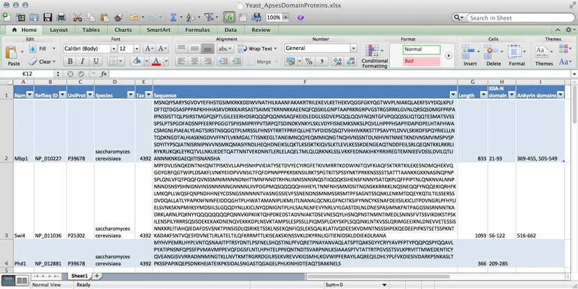
Many serious researchers keep their project data in spreadsheets. Often they use Excel, or an alternative like the free OpenOffice Calc, or Google Sheets, both of which are compatible with Excel and have some interesting advantages. Here, all your data is in one place, easy to edit. You can even do simple calculations - although you should never use Excel for statistics[8]. You could answer What percentage of my proteins have an Ankyrin domain? quite easily[9].
There are two major downsides to spreadsheets. For one, complex queries need programming. There is no way around this. You can program inside Excel with Visual Basic. But you might as well export your data so you can work on it with a "real" programming language. The other thing is that Excel does not scale very well. Once you have more than a hundred proteins in your spreadsheet, you can see how finding anything can become tedious.
However, just because it was built for business applications, and designed for use by office assistants, does not mean it is intrinsically unsuitable for our domain. It's important to be pragmatic, not dogmatic, when choosing tools: choose according to your real requirements. Sometimes "quick and dirty" is just fine, because quick.
R
R can keep complex data in data frames and lists. If we do data analysis with R, we have to load the data first. We can use any of the read.table() functions for structured data, read lines of raw text with readLines(), or slurp in entire files with scan(). But we could also keep the data in an R object in the first place that we can read from disk, analyze, modify, and write back. In this case, R becomes our database engine.
# Sample construction of an R database table as a dataframe

# Data for the Mbp1 protein
proteins <- data.frame(
    name     = "Mbp1",
    refSeq   = "NP_010227",
    uniProt  = "P39678",
    species  = "Saccharomyces cerevisiae",
    taxId    = "4392",
    sequence = paste(
                    "MSNQIYSARYSGVDVYEFIHSTGSIMKRKKDDWVNATHILKAANFAKAKR",
                    "TRILEKEVLKETHEKVQGGFGKYQGTWVPLNIAKQLAEKFSVYDQLKPLF",
                    "DFTQTDGSASPPPAPKHHHASKVDRKKAIRSASTSAIMETKRNNKKAEEN",
                    "QFQSSKILGNPTAAPRKRGRPVGSTRGSRRKLGVNLQRSQSDMGFPRPAI",
                    "PNSSISTTQLPSIRSTMGPQSPTLGILEEERHDSRQQQPQQNNSAQFKEI",
                    "DLEDGLSSDVEPSQQLQQVFNQNTGFVPQQQSSLIQTQQTESMATSVSSS",
                    "PSLPTSPGDFADSNPFEERFPGGGTSPIISMIPRYPVTSRPQTSDINDKV",
                    "NKYLSKLVDYFISNEMKSNKSLPQVLLHPPPHSAPYIDAPIDPELHTAFH",
                    "WACSMGNLPIAEALYEAGTSIRSTNSQGQTPLMRSSLFHNSYTRRTFPRI",
                    "FQLLHETVFDIDSQSQTVIHHIVKRKSTTPSAVYYLDVVLSKIKDFSPQY",
                    "RIELLLNTQDKNGDTALHIASKNGDVVFFNTLVKMGALTTISNKEGLTAN",
                    "EIMNQQYEQMMIQNGTNQHVNSSNTDLNIHVNTNNIETKNDVNSMVIMSP",
                    "VSPSDYITYPSQIATNISRNIPNVVNSMKQMASIYNDLHEQHDNEIKSLQ",
                    "KTLKSISKTKIQVSLKTLEVLKESSKDENGEAQTNDDFEILSRLQEQNTK",
                    "KLRKRLIRYKRLIKQKLEYRQTVLLNKLIEDETQATTNNTVEKDNNTLER",
                    "LELAQELTMLQLQRKNKLSSLVKKFEDNAKIHKYRRIIREGTEMNIEEVD",
                    "SSLDVILQTLIANNNKNKGAEQIITISNANSHA",
                    sep=""),
    seqLen   = 833,
    KilAN    = "21-93",
    Ankyrin  = "369-455, 505-549",
    stringsAsFactors = FALSE)

# add data for the Swi4 protein
proteins <- rbind(proteins,
                  data.frame(
    name     = "Swi4",
    refSeq   = "NP_011036",
    uniProt  = "P25302",
    species  = "Saccharomyces cerevisiae",
    taxId    = "4392",
    sequence = paste(
                    "MPFDVLISNQKDNTNHQNITPISKSVLLAPHSNHPVIEIATYSETDVYEC",
                    "YIRGFETKIVMRRTKDDWINITQVFKIAQFSKTKRTKILEKESNDMQHEK",
                    "VQGGYGRFQGTWIPLDSAKFLVNKYEIIDPVVNSILTFQFDPNNPPPKRS",
                    "KNSILRKTSPGTKITSPSSYNKTPRKKNSSSSTSATTTAANKKGKKNASI",
                    "NQPNPSPLQNLVFQTPQQFQVNSSMNIMNNNDNHTTMNFNNDTRHNLINN",
                    "ISNNSNQSTIIQQQKSIHENSFNNNYSATQKPLQFFPIPTNLQNKNVALN",
                    "NPNNNDSNSYSHNIDNVINSSNNNNNGNNNNLIIVPDGPMQSQQQQQHHH",
                    "EYLTNNFNHSMMDSITNGNSKKRRKKLNQSNEQQFYNQQEKIQRHFKLMK",
                    "QPLLWQSFQNPNDHHNEYCDSNGSNNNNNTVASNGSSIEVFSSNENDNSM",
                    "NMSSRSMTPFSAGNTSSQNKLENKMTDQEYKQTILTILSSERSSDVDQAL",
                    "LATLYPAPKNFNINFEIDDQGHTPLHWATAMANIPLIKMLITLNANALQC",
                    "NKLGFNCITKSIFYNNCYKENAFDEIISILKICLITPDVNGRLPFHYLIE",
                    "LSVNKSKNPMIIKSYMDSIILSLGQQDYNLLKICLNYQDNIGNTPLHLSA",
                    "LNLNFEVYNRLVYLGASTDILNLDNESPASIMNKFNTPAGGSNSRNNNTK",
                    "ADRKLARNLPQKNYYQQQQQQQQPQNNVKIPKIIKTQHPDKEDSTADVNI",
                    "AKTDSEVNESQYLHSNQPNSTNMNTIMEDLSNINSFVTSSVIKDIKSTPS",
                    "KILENSPILYRRRSQSISDEKEKAKDNENQVEKKKDPLNSVKTAMPSLES",
                    "PSSLLPIQMSPLGKYSKPLSQQINKLNTKVSSLQRIMGEEIKNLDNEVVE",
                    "TESSISNNKKRLITIAHQIEDAFDSVSNKTPINSISDLQSRIKETSSKLN",
                    "SEKQNFIQSLEKSQALKLATIVQDEESKVDMNTNSSSHPEKQEDEEPIPK",
                    "STSETSSPKNTKADAKFSNTVQESYDVNETLRLATELTILQFKRRMTTLK",
                    "ISEAKSKINSSVKLDKYRNLIGITIENIDSKLDDIEKDLRANA",
                    sep=""),
    seqLen   = 1093,
    KilAN    = "56-122",
    Ankyrin  = "516-662",
    stringsAsFactors = FALSE)
    )

# how many proteins?
nrow(proteins)

#what are their names?
proteins[,"name"]

# how many do not have an Ankyrin domain?
sum(proteins[,"Ankyrin"] == "")

# save it to file
save(proteins, file="proteinData.Rda")

# delete it from memory
rm(proteins)

# check...
proteins  # ... yes, it's gone


# read it back in:
load("proteinData.Rda")

# did this work?
sum(proteins[,"seqLen"])   # 1926 amino acids

# add another protein: Phd1
proteins <- rbind(proteins,
                  data.frame(
    name     = "Phd1",
    refSeq   = "NP_012881",
    uniProt  = "P39678",
    species  = "Saccharomyces cerevisiae",
    taxId    = "4392",
    sequence = paste(
                    "MPFDVLISNQKDNTNHQNITPISKSVLLAPHSNHPVIEIATYSETDVYEC",
                    "MYHVPEMRLHYPLVNTQSNAAITPTRSYDNTLPSFNELSHQSTINLPFVQ",
                    "RETPNAYANVAQLATSPTQAKSGYYCRYYAVPFPTYPQQPQSPYQQAVLP",
                    "YATIPNSNFQPSSFPVMAVMPPEVQFDGSFLNTLHPHTELPPIIQNTNDT",
                    "SVARPNNLKSIAAASPTVTATTRTPGVSSTSVLKPRVITTMWEDENTICY",
                    "QVEANGISVVRRADNNMINGTKLLNVTKMTRGRRDGILRSEKVREVVKIG",
                    "SMHLKGVWIPFERAYILAQREQILDHLYPLFVKDIESIVDARKPSNKASL",
                    "TPKSSPAPIKQEPSDNKHEIATEIKPKSIDALSNGASTQGAGELPHLKIN",
                    "HIDTEAQTSRAKNELS",
                    sep=""),
    seqLen   = 366,
    KilAN    = "209-285",
    Ankyrin  = "",    # No ankyrin domains annotated here
    stringsAsFactors = FALSE)
    )

# check:
proteins[,"name"]                #"Mbp1" "Swi4" "Phd1"
sum(proteins[,"Ankyrin"] == "")  # Now there is one...
sum(proteins[,"seqLen"])         # 2292 amino acids

# [END]
The third way to use R for data is to connect it to a "real" database:
- a relational database like mySQL, MariaDB, or PostgreSQL;
- an object/document database like {{WP|MongoDB};
- or even a graph-database like Neo4j.
R "drivers" are available for all of these. However all of these require installing extra software on your computer: the actual database, which runs as an independent application. If you need a rock-solid database with guaranteed integrity, industry standard performance, and scalability to even very large datasets and hordes of concurrent users, don't think of rolling your own solution. One of the above is the way to go.
MySQL and friends
MySQL is a free, open relational database that powers some of the largest corporations as well as some of the smallest laboratories. It is based on a client-server model. The database engine runs as a daemon in the background and waits for connection attempts. When a connection is established, the server process establishes a communication session with the client. The client sends requests, and the server responds. One can do this interactively, by running the client program /usr/local/mysql/bin/mysql (on Unix systems). Or, when you are using a program such as R, Python, Perl, etc. you use the appropriate method calls or functions—the driver—to establish the connection.
These types of databases use their own language to describe actions: SQL - which handles data definition, data manipulation, and data control.
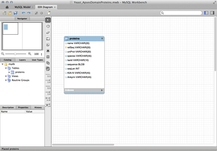
Just for illustration, the Figure above shows a table for our APSES domain protein data, built as a table in the MySQL workbench application and presented as an Entity Relationship Diagram (ERD). There is only one entity though - the protein "table". The application can generate the actual code that implements this model on a SQL compliant database:
CREATE TABLE IF NOT EXISTS `mydb`.`proteins` (
  `name` VARCHAR(20) NULL,
  `refSeq` VARCHAR(20) NOT NULL,
  `uniProt` VARCHAR(20) NULL,
  `species` VARCHAR(45) NOT NULL COMMENT '	',
  `taxId` VARCHAR(10) NULL,
  `sequence` BLOB NULL,
  `seqLen` INT NULL,
  `KilA-N` VARCHAR(45) NULL,
  `Ankyrin` VARCHAR(45) NULL,
  PRIMARY KEY (`refSeq`))
ENGINE = InnoDB
This looks at least as complicated as putting the model into R in the first place. Why then would we do this, if we need to load it into R for analysis anyway. There are several important reasons.
- Scalability: these systems are built to work with very large datasets and optimized for performance. In theory R has very good performance with large data objects, but not so when the data becomes larger than what the computer can keep in memory all at once.
- Concurrency: when several users need to access the data potentially at the same time, you must use a "real" database system. Handling problems of concurrent access is what they are made for.
- ACID compliance. ACID describes four aspects that make a database robust, these are crucial for situations in which you have only partial control over your system or its input, and they would be quite laborious to implement for your hand built R data model:
- Atomicity: Atomicity requires that each transaction is handled "indivisibly": it either succeeds fully, with all requested elements, or not at all.
- Consistency: Consistency requires that any transaction will bring the database from one valid state to another. In particular any data-validation rules have to be enforced.
- Isolation: Isolation ensures that any concurrent execution of transactions results in the exact same database state as if transactions would have been executed serially, one after the other.
- Durability: The Durability requirement ensures that a committed transaction remains permanently committed, even in the event that the database crashes or later errors occur. You can think of this like an "autosave" function on every operation.
All the database systems I have mentioned above are ACID compliant[10].
Data modelling
|
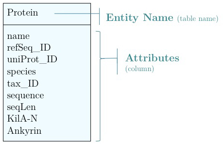
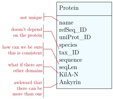
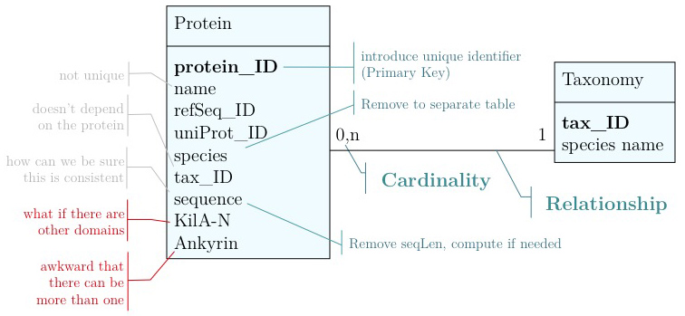
As you have seen above, the actual specification of a data model in R or as a sequence of SQL statements is quite technical and not well suited to obtain an overview for the model's main features that we would need for its design. We'll thus introduce a modelling convention: the Entity-Relationship Diagram (ERD). These are semi-formal diagrams that show the key features of the model. Currently we have only a single table defined, with a number of attributes. If we think a bit about our model and its intended use, it should become clear that there are a number of problems. They have to do with efficiency, and internal consistency. Problems include:
|
- Unique identifier
- Every entity in our data model should have its own, unique identifier. Typically this will simply be an integer that we should automatically increment with every new entry. Automatically. We have to be sure we don't make a mistake.
- Move species/tax_id to separate table
- If the relationship between two attributes does not actually depend on our protein, we move them to their own table. One identifier remains in our protein table. We call this a "foreign key". The relationship between the two tables is drawn as a line, and the cardinalities of the relationship are identified. "Cardinalities" means: how many entities of one table can be associated with one entity of the other table. Here,
0, non the left side means: a giventax_IDdoes not have to actually occur in the protein table i.e. we can put species in the table for which we actually have no proteins. There could also be many ("n") proteins for one species in our database. On the right hand side1means: there is exactly one species annotated for each protein. No more, no less.
- Remove redundant data
This is almost always a good idea. It's usually better just to compute seqLen or similar from the data. The exception is if something is expensive to compute and/or used often. Then we may store the reult in our datamodel, while making our procedures watertight so we store the correct values.
These are relatively easy repairs. Treating the domain annotations correctly requires a bit more surgery.
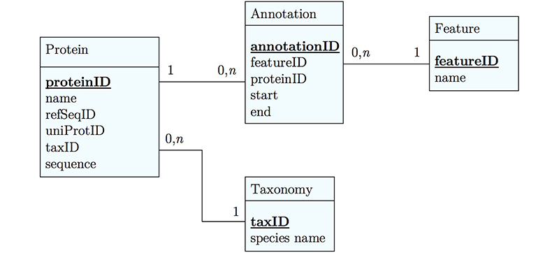
It's already awkward to work with a string like "21-93" when we need integer start and end values. We can parse them out, but it would be much more convenient if we can store them directly. But something like "369-455, 505-549" is really terrible. First of all it becomes an effort to tell how many domains there are in the first place, and secondly, the parsing code becomes quite involved. And that creates opportunities for errors in our logic and bugs in our code. And finally, what about if we have more features that we want to annotate? Should we have attributes like Kil-A N start, Kil-A N end, Ankyrin 01 start, Ankyrin 01 end, Ankyrin 02 start, Ankyrin 02 end, Ankyrin 03 start, Ankyrin 30 end... No, that would be absurdly complicated and error prone. There is a much better approach that solves all three problems at the same time. Just like with our species, we create a table that describes features. We can put any number of features there, even slightly different representations of canonical features from different data sources. Then we create a table that stores every feature occurrence in every protein. We call this a junction table and this is an extremely common pattern in data models. Each entry in this table links exactly one protein with exactly one feature. Each protein can have 0, n features. And each feature can be found in 0, n proteins.
With this simple schematic, we obtain an excellent overview about the logical structure of our data and how to represent it in code. Such models are essential for the design and documentation of any software project.
A System datamodel
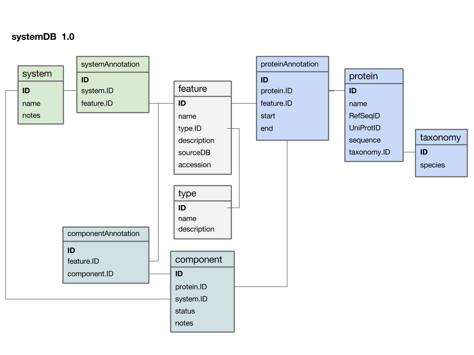
Here is a first version of a systems data model:
- The
featuretable is at the centre. This was not intentional, but emerged from iterating the model through a number of revisions. It emphasizes that the main purpose of this model is to integrate and annotate data from various sources. Feature in the way we understand it here is an abstraction of quite disparate categories of information items. This includes domain annotations, system functions, literature references, and cross-references to other databases. The type attribute will require some thought: this attribute really needs a "controlled vocabulary" to ensure that the same category is described consistently with the same string ("PubMed"? "Lit."? "reference"?). There are a number of ways to achieve this, the best way[11] is to store these types in their own "reference" tabletype- and link to that table via a foreign key. - The
proteintable is at the centre. Its primary key is a unique integer. We store the NCBI RefSeq ID and the Uniprot ID in the table. We would not call these "foreign keys", since the information they reference is not in our schema but at the NCBI resp. EBI. For example, we can't guarantee that they are unique keys. - The
taxonomytable holds information about species. We use the NCBI taxonomy ID as its primary key. The same key appears in the protein table as the foreign key that links the protein with its proper taxonomy information. This is an instance where the data model actually does not describe reality well. The problem is that particular proteins that we might retrieve from database searches will often be annotated to a specific strain of a species – and there is no easy way to reference strains to species. We'll see whether this turns out to be a problem in practice. But it may be that an additional table may be required that stores parent/child relationships of the taxonomic tree of life. - The
protein_featuretable links a protein with all the features that we annotate it with. start and end coordinates identify the region of the sequence we have annotated. - The
...Annotationtables link feature-information with annotated entities. - Should the
systemtable have its own taxonomy attribute? Or should the species in which the system is observed be inferred from the component protein'staxonomy.ID? What do you think? I decided not to add a taxonomy attribute to that table. How would you argue for or against this decision? - The
componenttable links proteins that collaborate together as a system. There is an implicit assumption in this model that only proteins are system components (and not e.g. RNA), and that components are atomic (i.e. we can't link to subsystems). How would you change the model to accommodate more realistic biological complexity?
Links and resources
| McInerny (2016) Cell cycle regulated transcription: from yeast to cancer. F1000Res 5:. (pmid: 27239285) |
|
[ PubMed ] [ DOI ] Recent studies have revealed exciting new functions for forkhead transcription factors in cell proliferation and development. Cell proliferation is a fundamental process controlled by multiple overlapping mechanisms, and the control of gene expression plays a major role in the orderly and timely division of cells. This occurs through transcription factors regulating the expression of groups of genes at particular phases of the cell division cycle. In this way, the encoded gene products are present when they are required. This review outlines recent advances in our understanding of this process in yeast model systems and describes how this knowledge has informed analysis in more developmentally complex eukaryotes, particularly where it is relevant to human disease. |
| McInerny (2011) Cell cycle regulated gene expression in yeasts. Adv Genet 73:51-85. (pmid: 21310294) |
|
[ PubMed ] [ DOI ] The regulation of gene expression through the mitotic cell cycle, so that genes are transcribed at particular cell cycle times, is widespread among eukaryotes. In some cases, it appears to be important for control mechanisms, as deregulated expression results in uncontrolled cell divisions, which can cause cell death, disease, and malignancy. In this review, I describe the current understanding of such regulated gene expression in two established simple eukaryotic model organisms, the budding yeast Saccharomyces cerevisiae and the fission yeast Schizosaccharomyces pombe. In these two yeasts, the global pattern of cell cycle gene expression has been well described, and most of the transcription factors that control the various waves of gene expression, and how they are in turn themselves regulated, have been characterized. As related mechanisms occur in all other eukaryotes, including humans, yeasts offer an excellent paradigm to understand this important molecular process. |
| Taylor et al. (2000) Characterization of the DNA-binding domains from the yeast cell-cycle transcription factors Mbp1 and Swi4. Biochemistry 39:3943-54. (pmid: 10747782) |
|
[ PubMed ] [ DOI ] The minimal DNA-binding domains of the Saccharomyces cerevisiae transcription factors Mbp1 and Swi4 have been identified and their DNA binding properties have been investigated by a combination of methods. An approximately 100 residue region of sequence homology at the N-termini of Mbp1 and Swi4 is necessary but not sufficient for full DNA binding activity. Unexpectedly, nonconserved residues C-terminal to the core domain are essential for DNA binding. Proteolysis of Mbp1 and Swi4 DNA-protein complexes has revealed the extent of these sequences, and C-terminally extended molecules with substantially enhanced DNA binding activity compared to the core domains alone have been produced. The extended Mbp1 and Swi4 proteins bind to their cognate sites with similar affinity [K(A) approximately (1-4) x 10(6) M(-)(1)] and with a 1:1 stoichiometry. However, alanine substitution of two lysine residues (116 and 122) within the C-terminal extension (tail) of Mbp1 considerably reduces the apparent affinity for an MCB (MluI cell-cycle box) containing oligonucleotide. Both Mbp1 and Swi4 are specific for their cognate sites with respect to nonspecific DNA but exhibit similar affinities for the SCB (Swi4/Swi6 cell-cycle box) and MCB consensus elements. Circular dichroism and (1)H NMR spectroscopy reveal that complex formation results in substantial perturbations of base stacking interactions upon DNA binding. These are localized to a central 5'-d(C-A/G-CG)-3' region common to both MCB and SCB sequences consistent with the observed pattern of specificity. Changes in the backbone amide proton and nitrogen chemical shifts upon DNA binding have enabled us to experimentally define a DNA-binding surface on the core N-terminal domain of Mbp1 that is associated with a putative winged helix-turn-helix motif. Furthermore, significant chemical shift differences occur within the C-terminal tail of Mbp1, supporting the notion of two structurally distinct DNA-binding regions within these proteins. |
| Deleeuw et al. (2008) Thermodynamics and specificity of the Mbp1-DNA interaction. Biochemistry 47:6378-85. (pmid: 18491920) |
|
[ PubMed ] [ DOI ] The DNA binding domain of the yeast transcription factor Mbp1 is a winged helix-turn-helix structure, with an extended DNA binding site involving C-terminal "tail" residues. The thermodynamics of the interaction of the DNA binding domain with its target DNA sequence have been determined using fluorescence anisotropy and calorimetry. The dissociation constant was determined as a function of pH and ionic strength in assessing the relative importance of specific and nonspecific ionic interactions. Mutational analysis of the residues in the binding site was used to determine their contributions to binding. The three tail histidine residues and His 63 in the recognition helix accounted for most of the pH dependence of the DNA binding. The tail histidine residues, along with two previously identified lysine residues, account for a major part of the polyelectrolyte contribution to binding and for the nonspecific affinity of Mbp1 for DNA. Gln67 was shown to be a very important residue, which interacts in the minor groove of the target DNA. Systematic mutations of the DNA consensus binding sites showed that the CGCG core contributes most to recognition. Isothermal titration calorimetry revealed a strong temperature-dependent enthalpy change, with a Delta Cp of -1.3kJ mol(-1) K(-1), consistent with a specific binding mode and burial of surface area. Parsing the free energy contributions demonstrates that polyelectrolyte effects account for half of the total free energy at the physiological pH and salt concentration. We present a model for the origin of the sequence specificity and overall affinity of the protein that accounts for the observed thermodynamics. |
- Further reading
| Chernatynskaya et al. (2009) Structural analysis of the DNA target site and its interaction with Mbp1. Org Biomol Chem 7:4981-91. (pmid: 19907790) |
|
[ PubMed ] [ DOI ] The solution structure of a 14 base-pair non-self complementary DNA duplex containing the consensus-binding site of the yeast transcription factor Mbp1 has been determined by NMR using a combination of scalar coupling analysis, time-dependent NOEs, residual dipolar couplings and 13C-edited NMR spectroscopy of a duplex prepared with one strand uniformly labeled with 13C-nucleotides. As expected, the free DNA duplex is within the B-family of structures, and within experimental limits is straight. However, there are clear local structural variations associated with the consensus CGCG element in the binding sequence that are important for sequence recognition. In the complex, the DNA bends around the protein, which also undergoes some conformational rearrangement in the C-terminal region. Structural constraints derived from paramagnetic perturbation experiments with spin-labeled DNA, chemical shift perturbation experiments of the DNA, previous cross-saturation, chemical shift perturbation experiments on the protein, information from mutational analysis, and electrostatics calculations have been used to produce a detailed docked structure using the known solution conformation of the free protein and other spectroscopic information about the Mbp1:DNA complex. A Monte Carlo-based docking procedure with restrained MD in a fully solvated system subjected to available experimental constraints produced models that account for the available structural data, and can rationalize the extensive thermodynamic data about the Mbp1:DNA complex. The protein:DNA interface is closely packed and is associated with a small number of specific contacts. The structure shows an extensive positively charged surface that accounts for the high polyelectrolyte contribution to binding. |
Footnotes and references
- ↑
McInerny (2011) Cell cycle regulated gene expression in yeasts. Adv Genet 73:51-85. (pmid: 21310294) [ PubMed ] [ DOI ] The regulation of gene expression through the mitotic cell cycle, so that genes are transcribed at particular cell cycle times, is widespread among eukaryotes. In some cases, it appears to be important for control mechanisms, as deregulated expression results in uncontrolled cell divisions, which can cause cell death, disease, and malignancy. In this review, I describe the current understanding of such regulated gene expression in two established simple eukaryotic model organisms, the budding yeast Saccharomyces cerevisiae and the fission yeast Schizosaccharomyces pombe. In these two yeasts, the global pattern of cell cycle gene expression has been well described, and most of the transcription factors that control the various waves of gene expression, and how they are in turn themselves regulated, have been characterized. As related mechanisms occur in all other eukaryotes, including humans, yeasts offer an excellent paradigm to understand this important molecular process.
- ↑
McInerny (2016) Cell cycle regulated transcription: from yeast to cancer. F1000Res 5:. (pmid: 27239285) [ PubMed ] [ DOI ] Recent studies have revealed exciting new functions for forkhead transcription factors in cell proliferation and development. Cell proliferation is a fundamental process controlled by multiple overlapping mechanisms, and the control of gene expression plays a major role in the orderly and timely division of cells. This occurs through transcription factors regulating the expression of groups of genes at particular phases of the cell division cycle. In this way, the encoded gene products are present when they are required. This review outlines recent advances in our understanding of this process in yeast model systems and describes how this knowledge has informed analysis in more developmentally complex eukaryotes, particularly where it is relevant to human disease.
- ↑ If you find this URL hard to remember, consider the acronyms:
- ncbi.nlm.nih.gov
- NCBI: National Center for Biotechnology Information
- NLM: National Library of Medicine
- NIH: National Institutes of Health
- GOV: the US GOVernment top-level domain
- ↑ When there is only a single match for a search, you will be been taken directly to the page.
- ↑ Actually the "real" SwissProt identifier would be patterned like
MBP1_YEAST.P39678is the corresponding UniProt identifier. - ↑ A good way to consolidate your knowledge is to summarize it for everyone on the Entrez page of the Student Wiki, or enhance the information you find there.
- ↑ Your operating system can help you keep the files organized. The "file system" is a database.
- ↑ For real: Excel is miserable and often wrong on statistics, and it makes horrible, ugly plots. See here and here why Excel problems are not merely cosmetic.
- ↑ At the bottom of the window there is a menu that says "sum = ..." by default. This provides simple calculations on the selected range. Set the choice to "count", select all Ankyrin domain entries, and the count shows you how many cells actually have a value.
- ↑ For a list of relational Database Management Systems, see here.
- ↑ Relational databases like MySQL, PostgresQL, and MariaDB offer the datatype "Enum" for this purpose but this is an inferior solution. Enum types need to be fixed at the time the schema is created, they can't store information about their semantics, i.e. how the keywords are defined and when they should be used, and they can't be used in more than one table, since they are metadata of one particular column.
Ask, if things don't work for you!
- If anything about this page is not clear to you, please ask on the mailing list. You can be certain that others will have had similar problems. Success comes from joining the conversation.
- Do consider how to ask your questions so that a meaningful answer is possible:
- Review Netiquette for the course mailing list.
- Read How to create a Minimal, Complete, and Verifiable example on stackoverflow and ...
- How to make a great R reproducible example.
| Data | Sequence | Structure | Phylogeny | Function |
