Difference between revisions of "Data modelling"
m (→R) |
m (→Data Modelling) |
||
| Line 295: | Line 295: | ||
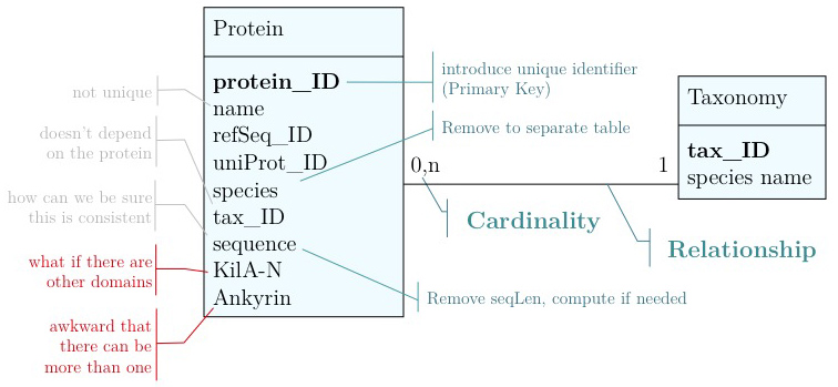
| + | [[Image:ERD_01.jpg|right|An ERD Diagram for our data model so far, the "attributes" for our ''Protein'' table are shown.]] | ||
| + | As you have seen above, the actual specification of a data model in '''R''' or as a sequence of SQL statements is quite technical and not well suited to obtain an overview for the model's main features that we would need for its design. We'll thus introduce a modelling convention: the '''Entity-Relationship Diagram (ERD)'''. These are semi-formal diagrams that show the key features of the model. Currently we have only a single table defined, with a number of attributes. | ||
| + | If we think a bit about our model and its intended use, it should become clear that there are a number of problems. They have to do with efficiency, and internal consistency. | ||
| + | |||
| + | |||
| + | [[Image:ERD_02.jpg|right|Problems with our data model.]] | ||
| + | |||
| + | |||
| + | Problems include: | ||
| + | *We don't have a unique identifier. The name "Mbp1" could appear more than once in our table. The database IDs for RefSeq and UniProt are unique (up to versions) but they mean something else and that can be very confusing. | ||
| + | *The relationship between species name and the taxonomy ID does not depend on the gene. In fact we could claim it to be different in different genes records. This would make our database inconsistent. | ||
| + | *We can't guarantee that the length of the sequence is correct, we might have made an error while updating. Since <code>seqLen</code> depends on the contents of <code>sequence</code> it is redundant to store it separately. | ||
| + | *A major issue is that we can't easily accommodate other features in our model. What about AT-hooks, disordered segments, phosphorylation sites, coiled-coil domains? ... <small>(It may be I know something you don't know, yet.)</small>. And what about different versions of the Kil-A N domain? Different databases annotate slightly different boundaries. | ||
| + | *The way we have treated the Ankyrin domain ranges so far is really awkward. We should be able to represent more than one domain in our model. | ||
| + | |||
| + | |||
| + | [[Image:ERD_03.jpg|right|A first set of changes.]] | ||
| + | ;Unique identifier | ||
| + | :Every entity in our data model should have its own, unique identifier. Typically this will simply be an integer that we should automatically increment with every new entry. Automatically. We have to be sure we don't make a mistake. | ||
| + | |||
| + | ;Move species/tax_id to separate table | ||
| + | :If the relationship between two attributes does not actually depend on our protein, we move them to their own table. One identifier remains in our protein table. We call this a "foreign key". The '''relationship''' between the two tables is drawn as a line, and the '''cardinalities''' of the relationship are identified. "Cardinalities" means: how many entities of one table can be associated with one entity of the other table. Here, <code>0, n</code> on the left side means: a given <code>tax_ID</code> does not have to actually occur in the protein table i.e. we can put species in the table for which we actually have no proteins. There could also be many ("n") proteins for one species in our database. On the right hand side <code>1</code> means: there is exactly one species annotated for each protein. No more, no less. | ||
| + | |||
| + | ;Remove redundant data | ||
| + | This is almost always a good idea. It's usually better just to compute <code>seqLen</code> or similar from the data. The exception is if something is expensive to compute and/or used often. Then we may store the reult in our datamodel, while making our procedures watertight so we store the correct values. | ||
| + | |||
| + | These are relatively easy repairs. Treating the domain annotations correctly requires a bit more surgery. | ||
| + | [[Image:ERD_03.jpg|right|An improved model of protein features. We store features in a table where we can describe them in general terms. We then create a separate table that annotates the start and end amino acid of each feature for a specific protein.]] | ||
| + | |||
| + | It's already awkward to work with a string like <code>"21-93"</code> when we need integer start and end values. We can parse them out, but it would be much more convenient if we can store them directly. But something like <code>"369-455, 505-549"</code> is really terrible. First of all it becomes an effort to tell how many domains there are in the first place, and secondly, the parsing code becomes quite involved. And that creates opportunities for errors in our logic and bugs in our code. And finally, what about if we have more features that we want to annotate? Should we have attributes like <code>Kil-A N start, Kil-A N end, Ankyrin 01 start, Ankyrin 01 end, Ankyrin 02 start, Ankyrin 02 end, Ankyrin 03 start, Ankyrin 30 end... </code> No, that would be absurdly complicated and error prone. There is a much better approach that solves all three problems at the same time. Just like with our species, we create a table that describes features. We can put any number of features there, even slightly different representations of canonical features from different data sources. Then we create a table that stores every '''feature occurrence''' in every protein. We call this a {{WP|junction table}} and this is an extremely common pattern in data models. | ||
| + | |||
| + | |||
| + | |||
| + | <section end=data_modelling /> | ||
| + | |||
| + | |||
| + | |||
| + | === ERD === | ||
Several variations on the technology to store data exist (see [http://en.wikipedia.org/wiki/Database the Wikipedia article]), here we will only consider the relational model that is accessed through the SQL (Structured Query Language). | Several variations on the technology to store data exist (see [http://en.wikipedia.org/wiki/Database the Wikipedia article]), here we will only consider the relational model that is accessed through the SQL (Structured Query Language). | ||
| Line 303: | Line 341: | ||
In principle, in a relational data model, data is organized in '''tables''' ('''entities''') that contain many '''rows''' ('''records''') each with a set of '''columns''' ('''attributes'''); a particular column of a particular row is a '''value'''. | In principle, in a relational data model, data is organized in '''tables''' ('''entities''') that contain many '''rows''' ('''records''') each with a set of '''columns''' ('''attributes'''); a particular column of a particular row is a '''value'''. | ||
| − | |||
Typically, a data model will capture descriptions of entities, their attributes and relationships. We therefore describe data in so called '''Entity-Relationship Diagrams''' (ERD), a schematic, high-level view of the world. ERDs are semi-formal, they include: | Typically, a data model will capture descriptions of entities, their attributes and relationships. We therefore describe data in so called '''Entity-Relationship Diagrams''' (ERD), a schematic, high-level view of the world. ERDs are semi-formal, they include: | ||
| Line 409: | Line 446: | ||
| | ||
| − | |||
=== Implementing: defining a schema === | === Implementing: defining a schema === | ||
Revision as of 07:21, 28 September 2015
Data modelling
The crucial first step of making real world biology computable is to define how we abstract properties, measure them and collect their values as data, store the data, and work with it.
Contents
- 1 Introductory reading
- 2 Data storage
- 3 Data Modelling
- 4 Installing MySQL
- 5 Perl DBI and DBD
- 6 Further reading
- 7 Notes
- 8 References
- 9 Further reading and resources
Related Pages
|
Introductory reading
Data storage
Any software project requires modelling on many levels - data-flow models, logic models, user interaction models and more. But all of these ultimately rely on a data model that defines how the world is going to be represented in the computer for the project's purpose. The process of abstraction of data entities and defining their relationships can (and should) take up a major part of the project definition, often taking several iterations until you get it right. Whether your data can be completely described, consistently stored and efficiently retrieved is determined to a large part by your data model.
Databases can take many forms, from memories in your brain, to shoe-cartons under your bed, to software applications on your computer, or warehouse-sized data centres. Fundamentally, these all do the same thing: collect information and make it available.
Let us consider collecting information on APSES-domain transcription factors in various fungi, with the goal of being able to compare them. Let's specify this as follows:
- cross reference the source databases;
- study if they have the same features (e.g. domains);
- and compare the features.
The underlying information can easily be retrieved for a protein from its RefSeq or UniProt entry.
Text files
A first attempt to organize the data might be simply to write it down in a large text file:
name: Mbp1
refseq ID: NP_010227
uniprot ID: P39678
species: Saccharomyces cerevisiae
taxonomy ID: 4392
sequence:
MSNQIYSARYSGVDVYEFIHSTGSIMKRKKDDWVNATHILKAANFAKAKR
TRILEKEVLKETHEKVQGGFGKYQGTWVPLNIAKQLAEKFSVYDQLKPLF
DFTQTDGSASPPPAPKHHHASKVDRKKAIRSASTSAIMETKRNNKKAEEN
QFQSSKILGNPTAAPRKRGRPVGSTRGSRRKLGVNLQRSQSDMGFPRPAI
PNSSISTTQLPSIRSTMGPQSPTLGILEEERHDSRQQQPQQNNSAQFKEI
DLEDGLSSDVEPSQQLQQVFNQNTGFVPQQQSSLIQTQQTESMATSVSSS
PSLPTSPGDFADSNPFEERFPGGGTSPIISMIPRYPVTSRPQTSDINDKV
NKYLSKLVDYFISNEMKSNKSLPQVLLHPPPHSAPYIDAPIDPELHTAFH
WACSMGNLPIAEALYEAGTSIRSTNSQGQTPLMRSSLFHNSYTRRTFPRI
FQLLHETVFDIDSQSQTVIHHIVKRKSTTPSAVYYLDVVLSKIKDFSPQY
RIELLLNTQDKNGDTALHIASKNGDVVFFNTLVKMGALTTISNKEGLTAN
EIMNQQYEQMMIQNGTNQHVNSSNTDLNIHVNTNNIETKNDVNSMVIMSP
VSPSDYITYPSQIATNISRNIPNVVNSMKQMASIYNDLHEQHDNEIKSLQ
KTLKSISKTKIQVSLKTLEVLKESSKDENGEAQTNDDFEILSRLQEQNTK
KLRKRLIRYKRLIKQKLEYRQTVLLNKLIEDETQATTNNTVEKDNNTLER
LELAQELTMLQLQRKNKLSSLVKKFEDNAKIHKYRRIIREGTEMNIEEVD
SSLDVILQTLIANNNKNKGAEQIITISNANSHA
length: 833
Kila-N domain: 21-93
Ankyrin domains: 369-455, 505-549

...
... and save it all in one large text file and whenever you need to look something up, you just open the file, look for e.g. the name of the protein and read what's there. Or - for a more structured approach, you could put this into several files in a folder.[1] This is a perfectly valid approach and for some applications it might not be worth the effort to think more deeply about how to structure the data, and store it in a way that it is robust and scales easily to large datasets. Alas, small projects have a tendency to grow into large projects and if you work in this way, it's almost guaranteed that you will end up doing many things by hand that could easily be automated. Imagine asking questions like:
- How many proteins do I have?
- What's the sequence of the Kila-N domain?
- What percentage of my proteins have an Ankyrin domain?
- Or two ...?
Answering these questions "by hand" is possible, but tedious.
Spreadsheets
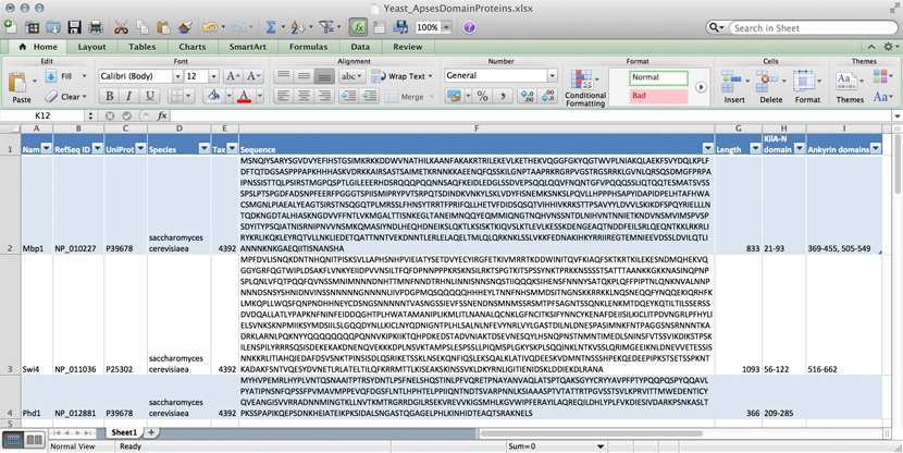
Many serious researchers keep their project data in spreadsheets. Often they use Excel, or an alternative like the free OpenOffice Calc, or Google Sheets, both of which are compatible with Excel and have some interesting advantages. Here, all your data is in one place, easy to edit. You can even do simple calculations - although you should never use Excel for statistics[2]. You could answer What percentage of my proteins have an Ankyrin domain? quite easily[3].
There are two major downsides to spreadsheets. For one, complex queries need programming. There is no way around this. You can program inside Excel with Visual Basic. But you might as well export your data so you can work on it with a "real" programming language. The other thing is that Excel does not scale very well. Once you have more than a hundred proteins in your spreadsheet, you can see how finding anything can become tedious.
However, just because it was built for business applications, and designed for use by office assistants, does not mean it is intrinsically unsuitable for our domain. It's important to be pragmatic, not dogmatic, when choosing tools: choose according to your real requirements. Sometimes "quick and dirty" is just fine, because quick.
R
R can keep complex data in data frames and lists. If we do data analysis with R, we have to load the data first. We can use any of the read.table() functions for structured data, read lines of raw text with readLines(), or slurp in entire files with scan(). But we could also keep the data in an R object in the first place that we can read from disk, analyze, modify, and write back. In this case, R becomes our database engine.
# Sample construction of an R database table as a dataframe

# Data for the Mbp1 protein
proteins <- data.frame(
    name     = "Mbp1",
    refSeq   = "NP_010227",
    uniProt  = "P39678",
    species  = "Saccharomyces cerevisiae",
    taxId    = "4392",
    sequence = paste(
                    "MSNQIYSARYSGVDVYEFIHSTGSIMKRKKDDWVNATHILKAANFAKAKR",
                    "TRILEKEVLKETHEKVQGGFGKYQGTWVPLNIAKQLAEKFSVYDQLKPLF",
                    "DFTQTDGSASPPPAPKHHHASKVDRKKAIRSASTSAIMETKRNNKKAEEN",
                    "QFQSSKILGNPTAAPRKRGRPVGSTRGSRRKLGVNLQRSQSDMGFPRPAI",
                    "PNSSISTTQLPSIRSTMGPQSPTLGILEEERHDSRQQQPQQNNSAQFKEI",
                    "DLEDGLSSDVEPSQQLQQVFNQNTGFVPQQQSSLIQTQQTESMATSVSSS",
                    "PSLPTSPGDFADSNPFEERFPGGGTSPIISMIPRYPVTSRPQTSDINDKV",
                    "NKYLSKLVDYFISNEMKSNKSLPQVLLHPPPHSAPYIDAPIDPELHTAFH",
                    "WACSMGNLPIAEALYEAGTSIRSTNSQGQTPLMRSSLFHNSYTRRTFPRI",
                    "FQLLHETVFDIDSQSQTVIHHIVKRKSTTPSAVYYLDVVLSKIKDFSPQY",
                    "RIELLLNTQDKNGDTALHIASKNGDVVFFNTLVKMGALTTISNKEGLTAN",
                    "EIMNQQYEQMMIQNGTNQHVNSSNTDLNIHVNTNNIETKNDVNSMVIMSP",
                    "VSPSDYITYPSQIATNISRNIPNVVNSMKQMASIYNDLHEQHDNEIKSLQ",
                    "KTLKSISKTKIQVSLKTLEVLKESSKDENGEAQTNDDFEILSRLQEQNTK",
                    "KLRKRLIRYKRLIKQKLEYRQTVLLNKLIEDETQATTNNTVEKDNNTLER",
                    "LELAQELTMLQLQRKNKLSSLVKKFEDNAKIHKYRRIIREGTEMNIEEVD",
                    "SSLDVILQTLIANNNKNKGAEQIITISNANSHA",
                    sep=""),
    seqLen   = 833,
    KilAN    = "21-93",
    Ankyrin  = "369-455, 505-549",
    stringsAsFactors = FALSE)

# add data for the Swi4 protein
proteins <- rbind(proteins,
                  data.frame(
    name     = "Swi4",
    refSeq   = "NP_011036",
    uniProt  = "P25302",
    species  = "Saccharomyces cerevisiae",
    taxId    = "4392",
    sequence = paste(
                    "MPFDVLISNQKDNTNHQNITPISKSVLLAPHSNHPVIEIATYSETDVYEC",
                    "YIRGFETKIVMRRTKDDWINITQVFKIAQFSKTKRTKILEKESNDMQHEK",
                    "VQGGYGRFQGTWIPLDSAKFLVNKYEIIDPVVNSILTFQFDPNNPPPKRS",
                    "KNSILRKTSPGTKITSPSSYNKTPRKKNSSSSTSATTTAANKKGKKNASI",
                    "NQPNPSPLQNLVFQTPQQFQVNSSMNIMNNNDNHTTMNFNNDTRHNLINN",
                    "ISNNSNQSTIIQQQKSIHENSFNNNYSATQKPLQFFPIPTNLQNKNVALN",
                    "NPNNNDSNSYSHNIDNVINSSNNNNNGNNNNLIIVPDGPMQSQQQQQHHH",
                    "EYLTNNFNHSMMDSITNGNSKKRRKKLNQSNEQQFYNQQEKIQRHFKLMK",
                    "QPLLWQSFQNPNDHHNEYCDSNGSNNNNNTVASNGSSIEVFSSNENDNSM",
                    "NMSSRSMTPFSAGNTSSQNKLENKMTDQEYKQTILTILSSERSSDVDQAL",
                    "LATLYPAPKNFNINFEIDDQGHTPLHWATAMANIPLIKMLITLNANALQC",
                    "NKLGFNCITKSIFYNNCYKENAFDEIISILKICLITPDVNGRLPFHYLIE",
                    "LSVNKSKNPMIIKSYMDSIILSLGQQDYNLLKICLNYQDNIGNTPLHLSA",
                    "LNLNFEVYNRLVYLGASTDILNLDNESPASIMNKFNTPAGGSNSRNNNTK",
                    "ADRKLARNLPQKNYYQQQQQQQQPQNNVKIPKIIKTQHPDKEDSTADVNI",
                    "AKTDSEVNESQYLHSNQPNSTNMNTIMEDLSNINSFVTSSVIKDIKSTPS",
                    "KILENSPILYRRRSQSISDEKEKAKDNENQVEKKKDPLNSVKTAMPSLES",
                    "PSSLLPIQMSPLGKYSKPLSQQINKLNTKVSSLQRIMGEEIKNLDNEVVE",
                    "TESSISNNKKRLITIAHQIEDAFDSVSNKTPINSISDLQSRIKETSSKLN",
                    "SEKQNFIQSLEKSQALKLATIVQDEESKVDMNTNSSSHPEKQEDEEPIPK",
                    "STSETSSPKNTKADAKFSNTVQESYDVNETLRLATELTILQFKRRMTTLK",
                    "ISEAKSKINSSVKLDKYRNLIGITIENIDSKLDDIEKDLRANA",
                    sep=""),
    seqLen   = 1093,
    KilAN    = "56-122",
    Ankyrin  = "516-662",
    stringsAsFactors = FALSE)
    )

# how many proteins?
nrow(proteins)

#what are their names?
proteins[,"name"]

# how many do not have an Ankyrin domain?
sum(proteins[,"Ankyrin"] == "")

# save it to file
save(proteins, file="proteinData.Rda")

# delete it from memory
rm(proteins)

# check...
proteins  # ... yes, it's gone


# read it back in:
load("proteinData.Rda")

# did this work?
sum(proteins[,"seqLen"])   # 1926 amino acids

# add another protein: Phd1
proteins <- rbind(proteins,
                  data.frame(
    name     = "Phd1",
    refSeq   = "NP_012881",
    uniProt  = "P39678",
    species  = "Saccharomyces cerevisiae",
    taxId    = "4392",
    sequence = paste(
                    "MPFDVLISNQKDNTNHQNITPISKSVLLAPHSNHPVIEIATYSETDVYEC",
                    "MYHVPEMRLHYPLVNTQSNAAITPTRSYDNTLPSFNELSHQSTINLPFVQ",
                    "RETPNAYANVAQLATSPTQAKSGYYCRYYAVPFPTYPQQPQSPYQQAVLP",
                    "YATIPNSNFQPSSFPVMAVMPPEVQFDGSFLNTLHPHTELPPIIQNTNDT",
                    "SVARPNNLKSIAAASPTVTATTRTPGVSSTSVLKPRVITTMWEDENTICY",
                    "QVEANGISVVRRADNNMINGTKLLNVTKMTRGRRDGILRSEKVREVVKIG",
                    "SMHLKGVWIPFERAYILAQREQILDHLYPLFVKDIESIVDARKPSNKASL",
                    "TPKSSPAPIKQEPSDNKHEIATEIKPKSIDALSNGASTQGAGELPHLKIN",
                    "HIDTEAQTSRAKNELS",
                    sep=""),
    seqLen   = 366,
    KilAN    = "209-285",
    Ankyrin  = "",    # No ankyrin domains annotated here
    stringsAsFactors = FALSE)
    )

# check:
proteins[,"name"]                #"Mbp1" "Swi4" "Phd1"
sum(proteins[,"Ankyrin"] == "")  # Now there is one...
sum(proteins[,"seqLen"])         # 2292 amino acids

# [END]
The third way to use R for data is to connect it to a "real" database:
- a relational database like mySQL, MariaDB, or PostgreSQL;
- an object/document database like {{WP|MongoDB};
- or even a graph-database like Neo4j.
R "drivers" are available for all of these. However all of these require installing extra software on your computer: the actual database, which runs as an independent application. If you need a rock-solid database with guaranteed integrity, industry standard performance, and scalability to even very large datasets and hordes of concurrent users, don't think of rolling your own solution. One of the above is the way to go.
MySQL and friends
MySQL is a free, open relational database that powers some of the largest corporations as well as some of the smallest laboratories. It is based on a client-server model. The database engine runs as a daemon in the background and waits for connection attempts. When a connection is established, the server process establishes a communication session with the client. The client sends requests, and the server responds. One can do this interactively, by running the client program /usr/local/mysql/bin/mysql (on Unix systems). Or, when you are using a program such as R, Python, Perl, etc. you use the appropriate method calls or functions—the driver—to establish the connection.
These types of databases use their own language to describe actions: SQL - which handles data definition, data manipulation, and data control.
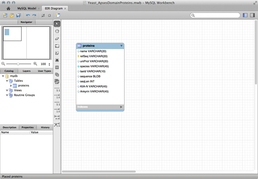
Just for illustration, the Figure above shows a table for our APSES domain protein data, built as a table in the MySQL workbench application and presented as an Entity Relationship Diagram (ERD). There is only one entity though - the protein "table". The application can generate the actual code that implements this model on a SQL compliant database:
CREATE TABLE IF NOT EXISTS `mydb`.`proteins` (
  `name` VARCHAR(20) NULL,
  `refSeq` VARCHAR(20) NOT NULL,
  `uniProt` VARCHAR(20) NULL,
  `species` VARCHAR(45) NOT NULL COMMENT '	',
  `taxId` VARCHAR(10) NULL,
  `sequence` BLOB NULL,
  `seqLen` INT NULL,
  `KilA-N` VARCHAR(45) NULL,
  `Ankyrin` VARCHAR(45) NULL,
  PRIMARY KEY (`refSeq`))
ENGINE = InnoDB
This looks at least as complicated as putting the model into R in the first place. Why then would we do this, if we need to load it into R for analysis anyway. There are several important reasons.
- Scalability: these systems are built to work with very large datasets and optimized for performance. In theory R has very good performance with large data objects, but not so when the data becomes larger than what the computer can keep in memory all at once.
- Concurrency: when several users need to access the data potentially at the same time, you must use a "real" database system. Handling problems of concurrent access is what they are made for.
- ACID compliance. ACID describes four aspects that make a database robust, these are crucial for situations in which you have only partial control over your system or its input, and they would be quite laborious to implement for your hand built R data model:
- Atomicity: Atomicity requires that each transaction is handled "indivisibly": it either succeeds fully, with all requested elements, or not at all.
- Consistency: Consistency requires that any transaction will bring the database from one valid state to another. In particular any data-validation rules have to be enforced.
- Isolation: Isolation ensures that any concurrent execution of transactions results in the exact same database state as if transactions would have been executed serially, one after the other.
- Durability: The Durability requirement ensures that a committed transaction remains permanently committed, even in the event that the database crashes or later errors occur. You can think of this like an "autosave" function on every operation.
All the database systems I have mentioned above are ACID compliant[4].
Data Modelling
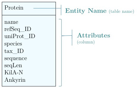
As you have seen above, the actual specification of a data model in R or as a sequence of SQL statements is quite technical and not well suited to obtain an overview for the model's main features that we would need for its design. We'll thus introduce a modelling convention: the Entity-Relationship Diagram (ERD). These are semi-formal diagrams that show the key features of the model. Currently we have only a single table defined, with a number of attributes.
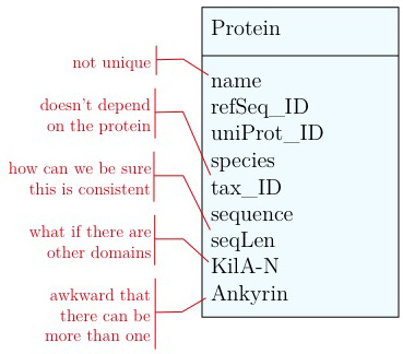
If we think a bit about our model and its intended use, it should become clear that there are a number of problems. They have to do with efficiency, and internal consistency.
Problems include:
- We don't have a unique identifier. The name "Mbp1" could appear more than once in our table. The database IDs for RefSeq and UniProt are unique (up to versions) but they mean something else and that can be very confusing.
- The relationship between species name and the taxonomy ID does not depend on the gene. In fact we could claim it to be different in different genes records. This would make our database inconsistent.
- We can't guarantee that the length of the sequence is correct, we might have made an error while updating. Since
seqLendepends on the contents ofsequenceit is redundant to store it separately. - A major issue is that we can't easily accommodate other features in our model. What about AT-hooks, disordered segments, phosphorylation sites, coiled-coil domains? ... (It may be I know something you don't know, yet.). And what about different versions of the Kil-A N domain? Different databases annotate slightly different boundaries.
- The way we have treated the Ankyrin domain ranges so far is really awkward. We should be able to represent more than one domain in our model.
- Unique identifier
- Every entity in our data model should have its own, unique identifier. Typically this will simply be an integer that we should automatically increment with every new entry. Automatically. We have to be sure we don't make a mistake.
- Move species/tax_id to separate table
- If the relationship between two attributes does not actually depend on our protein, we move them to their own table. One identifier remains in our protein table. We call this a "foreign key". The relationship between the two tables is drawn as a line, and the cardinalities of the relationship are identified. "Cardinalities" means: how many entities of one table can be associated with one entity of the other table. Here,
0, non the left side means: a giventax_IDdoes not have to actually occur in the protein table i.e. we can put species in the table for which we actually have no proteins. There could also be many ("n") proteins for one species in our database. On the right hand side1means: there is exactly one species annotated for each protein. No more, no less.
- Remove redundant data
This is almost always a good idea. It's usually better just to compute seqLen or similar from the data. The exception is if something is expensive to compute and/or used often. Then we may store the reult in our datamodel, while making our procedures watertight so we store the correct values.
These are relatively easy repairs. Treating the domain annotations correctly requires a bit more surgery.
It's already awkward to work with a string like "21-93" when we need integer start and end values. We can parse them out, but it would be much more convenient if we can store them directly. But something like "369-455, 505-549" is really terrible. First of all it becomes an effort to tell how many domains there are in the first place, and secondly, the parsing code becomes quite involved. And that creates opportunities for errors in our logic and bugs in our code. And finally, what about if we have more features that we want to annotate? Should we have attributes like Kil-A N start, Kil-A N end, Ankyrin 01 start, Ankyrin 01 end, Ankyrin 02 start, Ankyrin 02 end, Ankyrin 03 start, Ankyrin 30 end... No, that would be absurdly complicated and error prone. There is a much better approach that solves all three problems at the same time. Just like with our species, we create a table that describes features. We can put any number of features there, even slightly different representations of canonical features from different data sources. Then we create a table that stores every feature occurrence in every protein. We call this a junction table and this is an extremely common pattern in data models.
ERD
Several variations on the technology to store data exist (see the Wikipedia article), here we will only consider the relational model that is accessed through the SQL (Structured Query Language).
In principle, in a relational data model, data is organized in tables (entities) that contain many rows (records) each with a set of columns (attributes); a particular column of a particular row is a value.
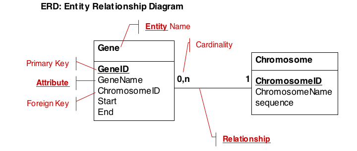
Typically, a data model will capture descriptions of entities, their attributes and relationships. We therefore describe data in so called Entity-Relationship Diagrams (ERD), a schematic, high-level view of the world. ERDs are semi-formal, they include:
- The entity (table) name
- Primary keys (use bold, underscore)
- All cardinalities
- All relationships
- The most important attributes (columns)
Normalization
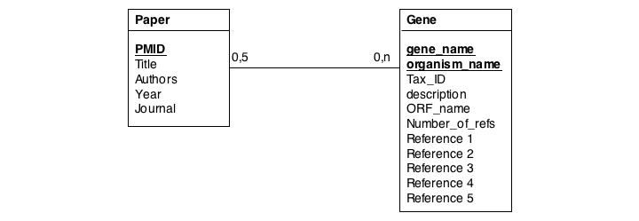
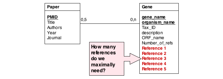
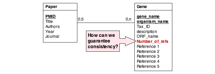
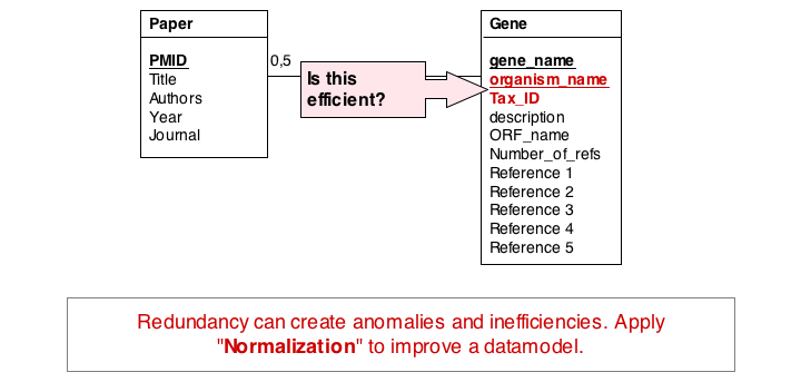
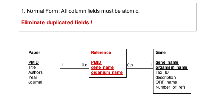
In this series of examples, we will discuss normalization of a simple data model that relates genes and publications that reference them. In a first attempt, we might define two tables: one contains data describing genes and one contains data describing a literature reference. Since there may be more than one publication referencing a gene, we provide for up to five references. We store the number of references a gene has in a separate column. We also store the organism name and the taxonomy ID in the gane table to identify the gene source. This model, while plausible on the surface, illustrates three common errors that can plague datamodeles.
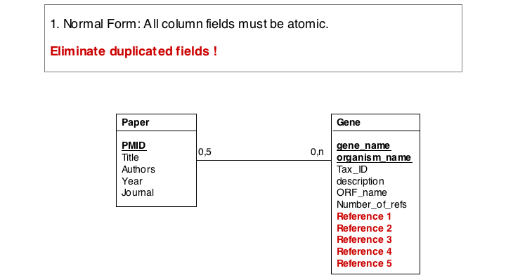
The first, and perhaps most obvious problem is the fact that we have stored several values of exactly the same type in the gene table. What happens if a gene has more than five references? This would break our model. And it is really inefficient to have to store null values whenever a gene has less than five references.
A more subtle problem arises when we store values that can be derived in an exact, functional way from the data that is stored: can we guarantee that the data is consistent? What happens if the value and the data somehow become inconsistent?
A third problem arises from storing the organism name and taxonomy ID in the gene table. Surely, the relationship between these two data items does not depend on which gene they are associated with. All three examples relate to unnecessary and redundant data that is not only inefficient to store but invites inconsistencies and is a potential source of errors in the database.
"Dependency theory" can be systematically applied to create efficient and consistent datamodels. The datamodel is brought into normal form. (See also the Wikipaedia article on database normalization.) As a principle, data should be stored only in one place in a database, and it should be stored in tables that are specific to that type of data.
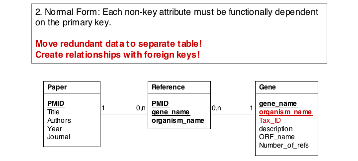
The soultion for the first problem is to eliminate the duplicated fields and store the related itmes in a separate table, a so called join table. In our example, each entry in the join table describes one reference to one particular gene. It is no problem at all to have the same paper talk about more than one gene, and it is easy to story any number of references to a gene in this table.
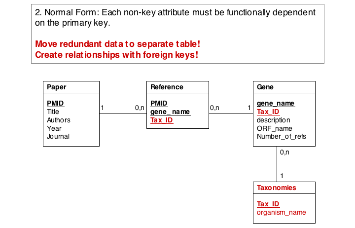
In the second form, we ensure a table stores only attributes of an entity that actually depend on the entity. In our example, organism_name and Tax_Id depend on each other, but not on the gene_name. It is sufficient to store eiether one of them with the gene_name. However, in practice abstract ID keys are usually preferred over keys that have semantics, such as a name or a date, simply because it is easy to keep an internal ID unique and usable as a key, but it may be hard to force the real world to behave in the same way. If two different organisms would have the same name, our model would break if we would rely on the name being unique.
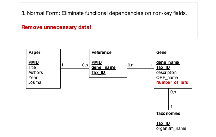
Finally, we eliminate evrything that does not need to be stored in the table, becausxe it can be computed from data in the table. For instance, the number of references for a gene can be easily obtained by an SQL select statement such as SELECT COUNT FROM Reference WHERE Reference.gene_name="Mbp1" AND 'Reference.Tax_ID="12345".
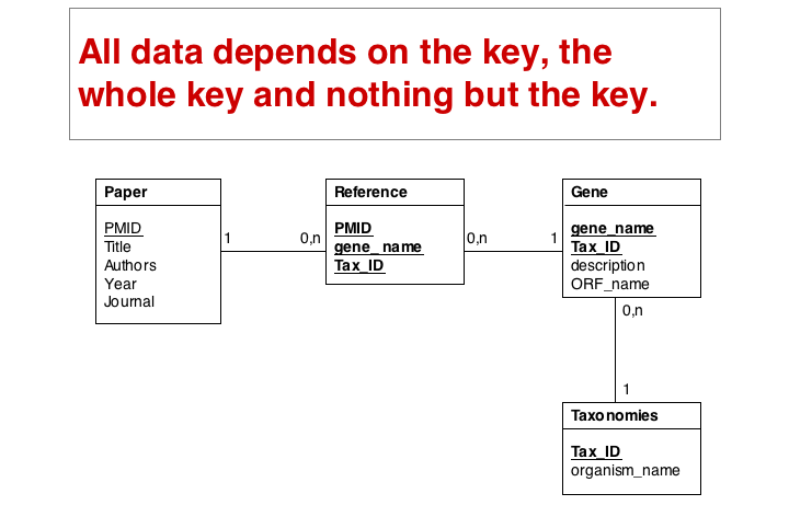
These operations finally give us the datamodel in 3. Normal Form. Note that for efficiency problems, datamodels may be intentionally denormalized: we may wish to store the results of expensive computations, for example, or we may store views (the results of SELECT operations) if they are complex and take a long time to ccompute, although the results could be derived from the data. However, such situations should never pass unintentionally and never undocumented.
Text
Implementing: defining a schema
While a database model such as the ERD describes the high-level intentions of the database, many additional decisions have to be taken before a model can actually be implemented. These concern the exact semantics (meaning) of components in the model, their datatypes and what to do in special circumstances (e.g.: whether a value is allowed to be undefined or NULL). We can document this information in a table, a database schema, as in the example below:
- Table - Database Schema Example showing the two tables from the model developed above.
| Table Name: Gene |
Semantics: A gene, its attributes and a reference to the chromosome table. |
||
| Column Name: | Type: | Properties: | Semantics: |
| Gene ID: | INT | PRIMARY KEY, AUTOINCREMENT, NOT NULL | Artificial key, no semantics outside of this database |
| Gene Name: | VARCHAR(10) | not NULL | The common name of the gene |
| Chromosome ID: | INT | Foreign Key, references Chromosome | References the Chromosome the gene is found on. Assumes a gene is found on exactly one Chromosome. |
| Start | INT | not NULL | Defines the first nucletodide (in chromosome coordinates) that is annotated as belonging to the gene. |
| End | INT | not NULL | Defines the last nucletodide (in chromosome coordinates) that is annotated as belonging to the gene. If End < Start, the gene is o the (-) strand. |
| Table Name: Chromosome |
Semantics: A chromosome, some attributes, and its sequence. |
||
| Column Name: | Type: | Properties: | Semantics: |
| Chromosome ID: | INT | PRIMARY KEY, AUTOINCREMENT, NOT NULL | Artificial key, no semantics outside of this database |
| Chromosome Name: | VARCHAR(10) | not NULL | The number/letter of the chromosome. Not required to be unique. |
| sequence | LONGTEXT | - | Holds the (+) strand sequence. Sequence defines chromosome coordinates. Gaps are filled with the character "N". |
As you design your schema, liberally enter comments for the table and each column. Don't describe what is there - that should be obvious - but why you have chosen to model it in this way and what consequences derive from the model. Describe what the columns mean in the real world, what their units of measurement are (if any) and what a NULL value means.
If you use an ENUM dta type, define all of its allowed values completely. Remeber that such a definition must be unique and complete: there may be no overlap between definitions and each conceivable object must correspond exactly to one enumerated value. Don't hesitate to use the term undefined as an option if you must defer the decision, but never let a gap in the decriptions pass.
If only a subset of integers are allowed, then document the allowed range in your schema. Some database will allow you to enter constraints that can be checked (although it may be desirable to enforce constraints at the aplication level).
Implementing: creating the database, importing data
To actually create the database, you have to cast the structure of your schema into a Data Definition Language (DDL), typically SQL. (See below.) A question that needs to be considered carefully is the degree to which processing logic should be delegated to the database, or handled by the application program (e.g. a Perl script). Often you will hear "Let the database do the work!". Obviously, the database is much better suited to e.g. perform a selection on items, a SELECT statement. It would not be sensible (albeit it is possible) to return the entire table instead and then filter records in the application program. However, this principle can be abused: a tendency to use overly specialized datatypes, an emphasis on stored procedures, or complicated output formatting by the database are in my mind often poor design choices for two reasons: one, you have to remember more than one way to achieve a desired result - in the database language as well as in the programming language, this may detract you from the task at hand and cause you to focus too much on the technology. The other is the question of documentation: if you use such sophistication, how do you make sure all the specifications are available and in synchrony with the code that uses and relies on them? It may be better to keep everything in one place, i.e. in your application program. That said, if many different programs need to access the same procedure, that one place may indeed be the database.
Database frontend
It is usually awkward to work with a database on the SQL commandline, although this is always possible. Usually the developer's work will include programming some database frontend to interact with the database, often these days this will be achieved through dynamic Web pages that show data on the page and allow to change data by submitting forms over the Web.
Installing MySQL
To install MySQL, follow this link for instructions.
Users, and The MySQL Privilege System
In order to actually do anything with your database, the appropriate access privileges must be in place. MySQL identifies you by the unique combination of username and hostname and associates your session with the appropriate SELECT, INSERT, UPDATE and DELETE privileges. At first, the server checks whether it can allow you to connect; subsequently it checks every single statement, whether it can allow you to execute it. The server stores all access information in tables in a database called mysql. These are the so-called grant tables.
You cannot view the grant table as a normal user, so for the following, please log in as the database administrator, root. The instructions how to secure the database by defining a root password were discussed on the installation page.
Please take care: as the administrator, you can ruin the database. Type the following carefully:
/usr/local/mysql/bin/mysql -u root -p
Enter password: ........
Welcome ... [...]
mysql> SHOW DATABASES;
+--------------------+
| Database           |
+--------------------+
| information_schema |
| mysql              |
| test               |
+--------------------+
3 rows in set (0.24 sec)
mysql> USE mysql;
Reading ... [...]
Database changed
mysql> SHOW TABLES;
+---------------------------+
| Tables_in_mysql           |
+---------------------------+
| columns_priv              |
| db                        |
| [...]                     |
| host                      |
| proc                      |
| procs_priv                |
| tables_priv               |
| [...]                     |
| user                      |
+---------------------------+
mysql> DESCRIBE user;
[...]
This lists all the various privileges that are stored in the user table. Lets see how many user identities have been created on the database:
mysql> SELECT Host, User, Password FROM user;
+----------------------------+------+-------------------------------------------+
| Host                       | User | Password                                  |
+----------------------------+------+-------------------------------------------+
| localhost                  | root | *852C5C17DEF9D1751FD661C1D0A0D48F4FC9DE91 |
| b-steipe01.med.utoronto.ca | root |                                           |
| b-steipe01.med.utoronto.ca |      |                                           |
| localhost                  |      |                                           |
+----------------------------+------+-------------------------------------------+
This shows an interesting inconsistency: I had secured the root user upon login from localhost, but not when I login from elsewhere. It also shows something useful: we might disallow root access from elsewhere, simply by refusing privileges to root@b-steipe01.med.utoronto.ca (or whatever your own version would be). For now, I fix the inconcistency by issuing the following statement on the commandline:
/usr/local/mysql/bin/mysqladmin -u root -h b-steipe01.med.utoronto.ca password ArarC0p_y
(or - directly from the mysql commandline (if you are logged in as root))
SET PASSWORD FOR 'root'@'b-steipe01.med.utoronto.ca' = PASSWORD('ArarC0p_y');
SET PASSWORD FOR @'b-steipe01.med.utoronto.ca' = PASSWORD('ArarC0p_y');
SET PASSWORD FOR @'localhost' = PASSWORD('ArarC0p_y');
etc.
Issuing the last SELECT statement again should show that the accounts now both require a password. Let us check on some of the relevant privileges:
mysql> SELECT Host, User, Select_priv, Delete_priv FROM user;
+----------------------------+------+-------------+-------------+
| Host                       | User | Select_priv | Delete_priv |
+----------------------------+------+-------------+-------------+
| localhost                  | root | Y           | Y           |
| b-steipe01.med.utoronto.ca | root | Y           | Y           |
| b-steipe01.med.utoronto.ca |      | N           | N           |
| localhost                  |      | N           | N           |
+----------------------------+------+-------------+-------------+
This is as expected: the root user is allowed to do things and everybody else is not. Of course, we don't want to login as root whenever we want to do anything with MySQL (nor would we want to store the root password in cleartext in our Perl sourcecode!), so we have to GRANT access privileges to normal users. As I wrote above, only the root user is allowed to do anything by default, the other users can only connect. However I also wrote that each and every single statement is evaluated for its privileges when it is being executed and thus we can GRANT privileges in a fine-grained way on a per-database, per-table and even per-column level. This is what the tables tables_priv and columns_priv are for. To summarize:
- The user table determines whether to reject or allow incoming connections. When a connection is allowed, any privileges granted in the user table applies to all databases on the server.
- The db table determines which users can access which databases from which hosts with which privileges. A privilege granted at the database level applies to the database and to all its tables. For example:
mysql> SELECT Host, Db, User, Select_priv FROM db;
+------+---------+------+-------------+
| Host | Db      | User | Select_priv |
+------+---------+------+-------------+
| %    | test    |      | Y           |
| %    | test\_% |      | Y           |
+------+---------+------+-------------+
... shows that the database "test", or any database with a name that starts with "test_" extends SELECT privileges to all users from any host.
- The tables_priv and columns_priv tables allow fine grained access. A privilege granted at the table level applies to the table and to all its columns. A privilege granted at the column level applies only to a specific column.
- As a consequence
- when playing around with code, simply call your database test_whatever and you can CREATE, ALTER and DROP it at will. For data that should persist, create the database as root then GRANT access privileges to whomever.
Reference
GRANTing privileges
In order to GRANT access, you have to CREATE a user, SET a PASSWORD and then GRANT privileges. Most commonly, you would grant a developer access to all functions of a database, then grant the Apache mysql client SELECT and maybe INSERT and UPDATE (as required) privileges... Still logged in as root I can issue the following statements:
mysql> CREATE DATABASE example;
mysql> GRANT ALL PRIVILEGES ON example.* TO 'developer'@'localhost'
    -> IDENTIFIED BY 'Nixo$poil' WITH GRANT OPTION;
mysql> show databases;
 [...]
mysql> SELECT Host,Db,User,Select_priv,Drop_priv FROM db WHERE Db='example';
+-----------+---------+-----------+-------------+-----------+
| Host      | Db      | User      | Select_priv | Drop_priv |
+-----------+---------+-----------+-------------+-----------+
| localhost | example | developer | Y           | Y         |
+-----------+---------+-----------+-------------+-----------+
This creates the user@host, sets the password and defines the privileges. The WITH GRANT OPTION statement ensures that developer can herself grant privileges to others: all privileges you have for a table can be granted to others, but only if this option is set.
In case you want to use the LOAD DATE INFILE option (discussed below) you have to also GRANT FILE privileges to your user. FILE privileges are administrative privileges and apply globally, not to only a single database. Therefore you have to grant them with a separate statement as follows:
mysql> GRANT FILE ON *.* TO 'developer'@'localhost' IDENTIFIED BY 'Nixo$poil' ;
(GRANTing to Apache will be discussed in our CGI introduction page).
Just one final warning. QUIT your root MySQL session now, then type
$ cat ~/.mysql_history
You may be surprised to find the password you have just entered for your new user to be shown in cleartext. This is a good time to check the privileges on this important file: they must be -rw-------.
Reference:
- TBC
Reference
- The MySQL account management syntax
- Adding New Users This is important - read about the distinction between localhost and other hosts.
Implementing a Physical Datamodel in MySQL
In SQL, the datamodel implementation is done with the CREATE DATABASE command, followed by the CREATE TABLE command. Each CREATE TABLE command contains information on all the columns of the table. Changes to the table are made with ALTER TABLE statments. A sample SQL session follows, to create the above example.
mysql> use example;
Database changed
mysql> CREATE TABLE Gene (
    -> Gene_ID INT NOT NULL PRIMARY KEY AUTO_INCREMENT,
    -> Gene_Name VARCHAR(10) NOT NULL,
    -> Chromosome_ID INT,
    -> Start INT NOT NULL,
    -> End INT NOT NULL
    -> );
Query OK, 0 rows affected (0.01 sec)

mysql> SHOW TABLES;
+-------------------+
| Tables_in_example |
+-------------------+
| Gene              |
+-------------------+
1 row in set (0.00 sec)

mysql> DESCRIBE Gene;
+---------------+-------------+------+-----+---------+----------------+
| Field         | Type        | Null | Key | Default | Extra          |
+---------------+-------------+------+-----+---------+----------------+
| Gene_ID       | int(11)     | NO   | PRI | NULL    | auto_increment |
| Gene_Name     | varchar(10) | NO   |     |         |                |
| Chromosome_ID | int(11)     | YES  |     | NULL    |                |
| Start         | int(11)     | NO   |     |         |                |
| End           | int(11)     | NO   |     |         |                |
+---------------+-------------+------+-----+---------+----------------+
5 rows in set (0.01 sec)

mysql>
MySQL Datatypes
It is important to give the datatypes some consideration since they influence not only what can be stored, searched and retrieved, but also how efficient the database stores data and how fast data-access is. Use the table below as a first reference (only selected types are included) and read up on details in the MySQL reference manual.
| Numeric Data | |
| BOOL | A Boolean value. Zero is FALSE, non-zero is TRUE. |
| INT | A normal (4byte, 32bit) integer. Range from 0 to 4,294,967,296 (unsigned, or half of that signed). |
| BIGINT | A double (8byte, 64bit) integer 0..~1.84*1019. |
| FLOAT | A single-precision (4byte, 32bit) floating point value. Range from +/- ~3*10+/- 38 with about 7 decimal places precision. Note that even though you may store single-precision floats, MySQL internally uses double precision and you may run into problems when you test for equality of two values. |
| DOUBLE | A normal, double-precision (8byte, 64bit) floating point value. Range from +/- ~1.8*10+/- 308 with approximately 15 decimal places precision. |
| String Data | |
| CHAR(n) | A fixed length string that is right-padded to n characters when stored. n is in the range 0..255. MySQL supports ASCII, UNICODE and national Character sets [1]. |
| VARCHAR(n) | A variable length string with a maximum length of n characters. |
| TEXT | A column with up to 65,535 text characters per field. TINYTEXT, MEDIUMTEXT and LONGTEXT are alternatives for different size storage requirements. |
| BLOB | A column with up to 65,535 bytes per field, useful e.g. to store images and other binary data. TINYBLOB, MEDIUMBLOB and LONGBLOB are alternatives for different size storage requirements. |
| ENUM | An enumeration of values - e.g ENUM ( 'value_1' , 'value_2' , 'value_3' , 'value_4' ) - useful to implement a constrained vocabulary. For example you might store status information for a process as ENUM ( 'pending' , 'executing' , 'aborted' , 'completed' ) |
| Time and Dates | |
| DATETIME | In 'YYYY-MM-DD HH:MM:SS' format (e.g. '2006-03-25 16:32:24). DATE and TIME are also available as separate types. |
| TIMESTAMP | A DATETIME value that is automatically set to the current time when the column is SET to a NULL value. |
| YEAR | A four-digit Year (1901-2155). Use of this specialized item (a 1 byte unsigned integer + 1900) is an example of design constraints that were more importnat when space and CPU cycles were very much more expensive than they are today. Don't fall into the trap of using a specialized type only because it exists, without proper consideration of the limitations this may impose. This is something we should have learned from the Y2K problem. |
NULL
The value NULL in MySQL deserves special mention. It is not equal to zero, nor is it FALSE. In fact, if you select from rows where values are TRUE, and then select values that are FALSE, the NULL values will be in neither selection. They only match the special expression "IS NULL". Undefined values will usually be set to NULL, except if a default value for the column has been defined. If the column has been created with the modifier "NOT NULL" an attempt at insertion of an undefined field will create an error.
Housekeeping
ALTER tables
Examples:
ALTER TABLE table RENAME new_table_name;
ALTER TABLE table ADD new_column_name data_type;
ALTER TABLE table CHANGE  column_name column_name new_data_type; (*)
ALTER TABLE table ALTER column_name SET DEFAULT new_value;
ALTER TABLE table DROP column_name;
(*) this is no typo: the column_name appears twice in this statement. The first time defines which column the statement applies to, the second time is part of the "create clause" that defines the change.
DROP tables or databases
Examples:
DROP TABLE table_name;
DROP DATABASE database_name;
Four important activities
SELECT
This is the main data-retrieval activity. Specified fields from records that match the selection criteria are sent to the client.
Examples:
SELECT column FROM table;
SELECT column_1,column_2 FROM table WHERE column_1= 'value' ;
SELECT column_1 FROM table_1, table_2 WHERE table_1.column_1=table_2.column_2;
INSERT
INSERT inserts a new row (record) into an existing table. Examples:
INSERT table_name (column_name) VALUES (value);
INSERT table_name (column_1, column_2) VALUES (value_1, value_2);
UPDATE
UPDATE changes values in an existing row (record). Examples:
UPDATE table_name SET column_name=value;
UPDATE table_name SET column_name=expression;  (e.g. ... SET Mol_weight=Mol_weight+116.23;)
UPDATE table_name SET column_name=value WHERE column_name=value;
DELETE
DELETE removes rows (records) from the database. Examples:
DELETE FROM table;   (Erases the entire table, but leaves its definition in place (as opposed to DROP ...))
DELETE FROM table WHERE column=value;
LOAD DATA INFILE
LOAD DATA INFILE can be used to import data into existing tables, IF for some obscure reason you can't have your own program code do this. By default (unless specified otherwise) the LOAD DATA statement works on tab-delimited, character containing (not binary) fields with newline-terminated records. Examples:
LOAD DATA INFILE filename INTO TABLE table;
LOAD DATA INFILE filename INTO TABLE table (column_1, column_2);
LOAD DATA INFILE filename INTO TABLE table (column_1, column_2) SET column_3=value;
Using mysqladmin for quick commandline database administration
The mysqladmin tool helps you with one-line administration tasks and is thus easy to use in scripts or cron-jobs. Examples:
/usr/local/mysql/bin/mysqladmin -u user password new_password
/usr/local/mysql/bin/mysqladmin version
/usr/local/mysql/bin/mysqladmin ping   (verifies that mysqld is running)
/usr/local/mysql/bin/mysqladmin reload  (reloads the grant tables)
/usr/local/mysql/bin/mysqladmin shutdown
Perl DBI and DBD
For a tutorial on embedding basic MySQL interactions into Perl programs, see the introduction to Perl and MySQL page.
Further reading
Notes
- ↑ Your operating system can help you keep the files organized. The "file system is a database.
- ↑ For real: Excel is miserable and often wrong on statistics, and it makes horrible, ugly plots. See here and here why Excel problems are not merely cosmetic.
- ↑ At the bottom of the window there is a menu that says "sum = ..." by default. This provides simple calculations on the selected range. Set the choice to "count", select all Ankyrin domain entries, and the count shows you how many cells actually have a value.
- ↑ For a list of relational Database Management Systems, see here.
References
Further reading and resources
