Difference between revisions of "Bioinformatics Introduction Function"

Latest revision as of 13:33, 9 January 2017

Function

Function

The Function Unit

This Unit is part of a brief introduction to bioinformatics. The material is more or less interleaved with the Function.R Project File which is part of the RStudio project associated with this material. Refer to the course/workshop page for installation instructions.

The unit covers expression analysis, introduces you to the STRING database of functional interactions, and explores graph analysis with the iGraph R package.

Expression Analysis

The transcriptome is the set of a cell's mRNA molecules. The transcriptome originates from the genome, mostly, that is, and it results in the proteome, again: mostly. RNA that is transcribed from the genome is not yet fit for translation but must be processed: splicing is ubiquitous^[1] and in addition RNA editing has been encountered in many species. Some authors therefore refer to the exome—the set of transcribed exons— to indicate the actual coding sequence.

Microarray technology — the quantitative, sequence-specific hybridization of labelled nucleotides in chip-format — was the first domain of "high-throughput biology". Today, it has largely been replaced by RNA-seq: quantification of transcribed mRNA by high-throughput sequencing and mapping reads to genes. Quantifying gene expression levels in a tissue-, development-, or response-specific way has yielded detailed insight into cellular function at the molecular level, with recent results of single-cell sequencing experiments adding a new level of precision. But not all transcripts are mapped to genes: we increasingly realize that the transcriptome is not merely a passive buffer of expressed information on its way to be translated into proteins, but contains multiple levels of complex, regulation through hybridization of small nuclear RNAs^[2].

In this unit, we will look at differential expression of Mbp1 and its target genes.

GEO2R

In this exercise we will use the analysis facilities of the GEO database at the NCBI.

Task:

First, we will search for relevant data sets on GEO, the NCBI's database for expression data.

Navigate to the entry page for GEO data sets].
Enter the following query in the usual Entrez query format: "cell cycle"[ti] AND "saccharomyces cerevisiae"[organism].
You should get two datasets among the top hits that analyze wild-type yeast (W303a cells) across two cell-cycles after release from alpha-factor arrest. Choose the experiment with lower resolution (13 samples).
On the linked GEO DataSet Browser page, follow the link to the Accession Viewer page: the "Reference series".
Read about the experiment and samples, then follow the link to analyze with GEO2R

View the GEO2R video tutorial on youtube.

Now proceed to apply this to the yeast cell-cycle study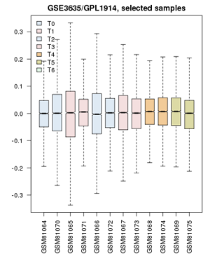: Value distribution for the yeast cell-cycle experiment GSE3635. Experiments are grouped approximately into equivalent time-points on a cell cycle.

Define groups: the associated publication shows us that one cell-cycle takes pretty exactly 60 minutes. Create timepoints T0, T1, T2, ... T5. Then associate the 0 and 60 min. sample with "T0"; 10 and 70 minutes get grouped as "T1"; 20 and 80 minutes are T2, etc. up to T5. The final sample does not get assigned.
Confirm that the Value distributions are unbiased by accessing the value distribution tab - overall, in such experiments, the bulk of the expression values should not change and thus means and quantiles of the expression levels should be about the same.
Your distribution should look like the image on the right: properly grouped into six categories, and unbiased regarding absolute expression levels and trends.
Look for differentially expressed genes: open the GEO2R tab and click on Top 250.

Analyze the results.

Examine the top hits. Click on a few of the gene names in the Gene.symbol column to view the expression profiles that tell you why the genes were found to be differentially expressed. What do you think? Is this what you would have expected for genes' responses to the cell-cycle? What seems to be the algorithm's notion of what "differentially expressed" means?
Look for expected genes. Here are a few genes that are known to be differentially expressed in the cell-cycle as target genes of the MBF complex: DSE1, DSE2, ERF3, HTA2, HTB2, and GAS3. But what about the MBD complex proteins themselves: Mbp1 and Swi6?

The notion of "differential expression" and "cell-cycle dependent expression" do not overlap completely. Significant differential expression is mathematically determined for genes that have low variance within groups and large differences between groups. This algorithm has no notion of any expectation you might have about the shape of the expression profile. All it finds are genes for which differential expression between some groups is statistically supported. The algorithm returns the top 250 of those. Consistency within groups is very important, while we intuitively might be giving more weight to conformance to our expectations of a cyclical pattern.

Let's see if we can group our time points differently to enhance the contrast between expression levels for cyclically expressed genes. Let's define only two groups: one set before and between the two cycles, one set at the peaks - and we'll omit some of the intermediate values.

Remove all of your groups and define two groups only. Call them "A" and "B".
Assign samples for T = 0 min, 10, 60 and 70 min. to the "A" group. Assign sets 30, 40, 90, and 100 to the "B" group.
Recalculate the Top 250 differentially expressed genes (you might have to refresh the page to get the "Top 250" button back.) Which of the "known" MBF targets are now contained in the set? What about Mbp1 and Swi6?
Finally: Let's compare the expression profiles for Mbp1, Swi6 and Swi4. It is not obvious that transcription factors are themselves under transcriptional control, as opposed to being expressed at a basal level and activated by phosporylation or ligand binding. In a new page, navigate to the Geo profiles page and enter (Mbp1 OR Swi6 OR Swi4 OR Nrm1 OR Cln1 OR Clb6 OR Act1 OR Alg9) AND GSE3635 (Nrm1, Cln1, and Clb6 are Mbp1 target genes. Act1 and Alg9 are beta-Actin and mannosyltransferase, these are often used as "housekeeping genes, i.e. genes with condition-independent expression levels, especially for qPCR studies - although Alg9 is also an Mbp1 target. We include them here as negative controls. CGSE3635 is the ID of the GEO data set we have just studied). You could have got similar results in the Profile graph tab of the GEO2R page. What do you find? What does this tell you? Would this information allow you to define groups that are even better suited for finding cyclically expressed genes?
Click on the profile graph for Mbp1 and print out the page. I may ask you to hand in this page for credit in the course. With a red pen, in one sentence describe the evidence you find on that page that allows us to conclude whether or not Mbp1 is a cell-cycle gene. You'll probably want to think for a moment what this question really means, how a cell-cycle gene could be defined, and what can be considered "evidence", before you write.

Protein-Protein Interactions

Task:

Study these lecture notes that are relevant for this unit Week 11: Annotated Notes (PDF 12.2 MB).

For a useful overview of graph-theory concepts, please read:

Pavlopoulos et al. (2011) Using graph theory to analyze biological networks. BioData Min 4:10. (pmid: 21527005)

[ PubMed ] [ DOI ] Understanding complex systems often requires a bottom-up analysis towards a systems biology approach. The need to investigate a system, not only as individual components but as a whole, emerges. This can be done by examining the elementary constituents individually and then how these are connected. The myriad components of a system and their interactions are best characterized as networks and they are mainly represented as graphs where thousands of nodes are connected with thousands of vertices. In this article we demonstrate approaches, models and methods from the graph theory universe and we discuss ways in which they can be used to reveal hidden properties and features of a network. This network profiling combined with knowledge extraction will help us to better understand the biological significance of the system.

Data Sources

Interaction databases have similar problems as sequence databases: the need for standards for abstracting biological concepts into computable objects, data integrity, search and retrieval, and the metrics of comparison. There is however an added complication: interactions are rarely all-or-none, and the high-throughput experimental methods have large false-positive and false-negative rates. This makes it necessary to define confidence scores for interactions. On top of experimental methods, there are also a variety of methods for computational interaction prediction. However, even though the "gold standard" are careful, small-scale laboratory experiments, different curated efforts on the same experimental publication usually lead to different results - with as little as 42% overlap between databases being reported.

Currently, likely the best integrated protein-protein interaction database is IntAct, at the EBI, which besides curating interactions from the literature hosts interactions from the IMEx consortium, an extensive data-sharing agreement between a number of general and specialized source databases.

Task:

Access IntAct and enter the UniProt ID for yeast Mbp1 P39678.
Click on the "Graph" tab to load a network graph.
Switch "Merge edges" off to show the reported edges for this interaction individually. Which protein pair has the most interactions? Does this make sense?

But then what?

If you are like me, you would now like to be able to link expression profiles, information about known complexes, GO annotations, knock-out phenotypes etc. etc. Too bad.

Interaction data visualization and analysis

If you work a lot with interaction networks, sooner or later you will come across Cytoscape. It is more or less the standard among "professional" systems biologists. But it is not an online tool.

Task:

Navigate to the Cytoscape homepage and inform yourself what the program does and how to install it. There are many tutorials online available. But this is software that needs to be downloaded, and installed and it definitively has a learning curve.

The state of integrated online interaction viewers these days could be improved. Have a look at this article that discusses the gap between what one would need to do, and what is offered:

Jeanquartier et al. (2015) Integrated web visualizations for protein-protein interaction databases. BMC Bioinformatics 16:195. (pmid: 26077899)

[ PubMed ] [ DOI ] BACKGROUND: Understanding living systems is crucial for curing diseases. To achieve this task we have to understand biological networks based on protein-protein interactions. Bioinformatics has come up with a great amount of databases and tools that support analysts in exploring protein-protein interactions on an integrated level for knowledge discovery. They provide predictions and correlations, indicate possibilities for future experimental research and fill the gaps to complete the picture of biochemical processes. There are numerous and huge databases of protein-protein interactions used to gain insights into answering some of the many questions of systems biology. Many computational resources integrate interaction data with additional information on molecular background. However, the vast number of diverse Bioinformatics resources poses an obstacle to the goal of understanding. We present a survey of databases that enable the visual analysis of protein networks. RESULTS: We selected M=10 out of N=53 resources supporting visualization, and we tested against the following set of criteria: interoperability, data integration, quantity of possible interactions, data visualization quality and data coverage. The study reveals differences in usability, visualization features and quality as well as the quantity of interactions. StringDB is the recommended first choice. CPDB presents a comprehensive dataset and IntAct lets the user change the network layout. A comprehensive comparison table is available via web. The supplementary table can be accessed on http://tinyurl.com/PPI-DB-Comparison-2015. CONCLUSIONS: Only some web resources featuring graph visualization can be successfully applied to interactive visual analysis of protein-protein interaction. Study results underline the necessity for further enhancements of visualization integration in biochemical analysis tools. Identified challenges are data comprehensiveness, confidence, interactive feature and visualization maturing.

The online resource that comes out as the best is the one at the String database.

Task:

Navigate to the String database and search for saccharomyces cerevisiae Mbp1 interactors.
Visualize the network. Add a few proteins by clicking the (+) button a two or three times.
Click on a node to get a synopsis of its function.
Explore the "confidence", "evidence" and "actions" networks for the retrieved interactors.
Not all interacting proteins are also predicted to have a functional relationship with Mbp1. Do you agree?
Explore the clustering and layout options. Do you understand what they do?
Explore the Views on

Neighborhood (not relevant for our query though)
Fusion (also not relevant for our query)
Occurence
Coexpression
Experiments
Database, and
Textmining

Each of these are methods for predicting functional relationships. Figure out how each one contributes to evidence of a functional interaction between Mbp1 and its predicted functional partners. I find the Occurrence view a unique and intriguing tool: visualizing in which organisms groups of genes are either all absent or all present allows to quickly establish functional clusters.

In summary, STRING is a convincingly well built tool to explore functional relationships between proteins.

Working with biological graphs in R

Task:

Open RStudio.
Choose File → Recent Projects → R-Exercise_Bioinformatics.
Pull the latest version of the project repository from GitHub.
type init()
Open the file Function.R and work through the entire tutorial.

At the end of the tutorial, you are being asked to print R code and data on a sheet of paper. I may ask you to hand this in for credit later in the course.

Links and resources

Barrett et al. (2013) NCBI GEO: archive for functional genomics data sets--update. Nucleic Acids Res 41:D991-5. (pmid: 23193258)

[ PubMed ] [ DOI ] The Gene Expression Omnibus (GEO, http://www.ncbi.nlm.nih.gov/geo/) is an international public repository for high-throughput microarray and next-generation sequence functional genomic data sets submitted by the research community. The resource supports archiving of raw data, processed data and metadata which are indexed, cross-linked and searchable. All data are freely available for download in a variety of formats. GEO also provides several web-based tools and strategies to assist users to query, analyse and visualize data. This article reports current status and recent database developments, including the release of GEO2R, an R-based web application that helps users analyse GEO data.

Okamura et al. (2015) COXPRESdb in 2015: coexpression database for animal species by DNA-microarray and RNAseq-based expression data with multiple quality assessment systems. Nucleic Acids Res 43:D82-6. (pmid: 25392420)

[ PubMed ] [ DOI ] The COXPRESdb (http://coxpresdb.jp) provides gene coexpression relationships for animal species. Here, we report the updates of the database, mainly focusing on the following two points. For the first point, we added RNAseq-based gene coexpression data for three species (human, mouse and fly), and largely increased the number of microarray experiments to nine species. The increase of the number of expression data with multiple platforms could enhance the reliability of coexpression data. For the second point, we refined the data assessment procedures, for each coexpressed gene list and for the total performance of a platform. The assessment of coexpressed gene list now uses more reasonable P-values derived from platform-specific null distribution. These developments greatly reduced pseudo-predictions for directly associated genes, thus expanding the reliability of coexpression data to design new experiments and to discuss experimental results.

Pavlopoulos et al. (2011) Using graph theory to analyze biological networks. BioData Min 4:10. (pmid: 21527005)

[ PubMed ] [ DOI ] Understanding complex systems often requires a bottom-up analysis towards a systems biology approach. The need to investigate a system, not only as individual components but as a whole, emerges. This can be done by examining the elementary constituents individually and then how these are connected. The myriad components of a system and their interactions are best characterized as networks and they are mainly represented as graphs where thousands of nodes are connected with thousands of vertices. In this article we demonstrate approaches, models and methods from the graph theory universe and we discuss ways in which they can be used to reveal hidden properties and features of a network. This network profiling combined with knowledge extraction will help us to better understand the biological significance of the system.

Footnotes and references

↑ Strictly speaking, splicing is an eukaryotic achievement, however there are examples of splicing in prokaryotes as well.
↑
(2015) The noncoding explosion. Nat Struct Mol Biol 22:1. (pmid: 25565024)

[ PubMed ] [ DOI ]

Jarvis & Robertson (2011) The noncoding universe. BMC Biol 9:52. (pmid: 21798102)

[ PubMed ] [ DOI ]

Ask, if things don't work for you!

If anything about this page is not clear to you, please ask on the mailing list. You can be certain that others will have had similar problems. Success comes from joining the conversation.

Do consider how to ask your questions so that a meaningful answer is possible:
- Review Netiquette for the course mailing list.
- Read How to create a Minimal, Complete, and Verifiable example on stackoverflow and ...
- How to make a great R reproducible example.

Function

[1] Strictly speaking, splicing is an eukaryotic achievement, however there are examples of splicing in prokaryotes as well.

[2] 
(2015) The noncoding explosion. Nat Struct Mol Biol 22:1. (pmid: 25565024)

[ PubMed ] [ DOI ]

Jarvis & Robertson (2011) The noncoding universe. BMC Biol 9:52. (pmid: 21798102)

[ PubMed ] [ DOI ]

[1]

[2]

Difference between revisions of "Bioinformatics Introduction Function"

Latest revision as of 13:33, 9 January 2017

Contents

The Function Unit

Expression Analysis

GEO2R

Protein-Protein Interactions

Data Sources

Interaction data visualization and analysis

Working with biological graphs in R

Links and resources

Footnotes and references

Ask, if things don't work for you!

Navigation menu

Personal tools

Namespaces

Variants

Views

More

Search

Sections

Tools

@@ Line 12: / Line 12: @@
 </tr></table>
+{{Vspace}}
+{{Vspace}}
 __TOC__
+{{Vspace}}
+==The Function Unit==
+This Unit is part of a brief introduction to bioinformatics. The material is more or less interleaved with the <code>Function.R</code> Project File which is part of the RStudio project associated with this material. Refer to the course/workshop page for installation instructions.
+The unit covers expression analysis, introduces you to the STRING database of functional interactions, and explores graph analysis with the iGraph '''R''' package.
+{{Vspace}}
+{{Vspace}}
 ==Expression Analysis==
@@ Line 24: / Line 38: @@
 '''Microarray technology''' &mdash; the quantitative, sequence-specific hybridization of labelled nucleotides in chip-format &mdash; was the first domain of "high-throughput biology". Today, it has largely been replaced by {{WP|RNA-Seq|'''RNA-seq'''}}: quantification of transcribed mRNA by high-throughput sequencing and mapping reads to genes. Quantifying gene expression levels in a  tissue-, development-, or response-specific way has yielded detailed insight into cellular function at the molecular level, with recent results of single-cell sequencing experiments adding a new level of precision. But not all transcripts are mapped to genes: we increasingly realize that the transcriptome is not merely a passive buffer of expressed information on its way to be translated into proteins, but contains multiple levels of complex, regulation through hybridization of small nuclear RNAs<ref>{{#pmid: 25565024}} {{#pmid: 21798102}}</ref>.
-In this assignment, we will look at differential expression of Mbp1 and its target genes.
+In this unit, we will look at differential expression of Mbp1 and its target genes.
+{{Vspace}}
-&nbsp;
+===GEO2R===
-==GEO2R==
 <section begin=exercises />
@@ Line 66: / Line 79: @@
 # Recalculate the '''Top 250''' differentially expressed genes (you might have to refresh the page to get the "Top 250" button back.) Which of the "known" MBF targets are now contained in the set? What about Mbp1 and Swi6?
 # Finally: Let's compare the expression profiles for Mbp1, Swi6 and Swi4. It is not obvious that transcription factors are themselves under '''transcriptional''' control, as opposed to being expressed at a basal level and ''activated'' by phosporylation or ligand binding. In a new page, navigate to the [http://www.ncbi.nlm.nih.gov/geoprofiles '''Geo profiles'''] page and enter <code>(Mbp1 OR Swi6 OR Swi4 OR Nrm1 OR Cln1 OR Clb6 OR Act1 OR Alg9) AND GSE3635</code> (Nrm1, Cln1, and Clb6 are Mbp1 target genes. Act1 and Alg9 are beta-Actin and mannosyltransferase, these are often used as "housekeeping genes, i.e. genes with condition-independent expression levels, especially for qPCR studies - although Alg9 is also an Mbp1 target. We include them here as negative controls. CGSE3635 is the ID of the GEO data set we have just studied). You could have got similar results in the '''Profile graph''' tab of the GEO2R page. What do you find? What does this tell you? Would this information allow you to define groups that are even better suited for finding cyclically expressed genes?
-# Click on the profile graph for Mbp1 and print out the page. Write your name and student number on the page. With a red pen, '''in one sentence''' describe the evidence you find '''on that page''' that allows us to conclude '''whether or not''' Mbp1 is a cell-cycle gene. You'll probably want to think for a moment what this question really means, how a cell-cycle gene could be defined, and what can be considered "evidence", before you write. I will mark your response for a maximum of four marks.
+# Click on the profile graph for Mbp1 and print out the page. I may ask you to hand in this page for credit in the course. With a red pen, '''in one sentence''' describe the evidence you find '''on that page''' that allows us to conclude '''whether or not''' Mbp1 is a cell-cycle gene. You'll probably want to think for a moment what this question really means, how a cell-cycle gene could be defined, and what can be considered "evidence", before you write.
   <!--
 * Finally, review the '''R''' script for the GEO2R analysis in the '''R script''' tab. This code will run on your machine and make the expression analysis available. Once the datasets are loaded and prepared, you could - for example - perform a "real" time series analysis, calculate correlation coefficients with an idealized sine wave, or search for genes that are '''co-regulated''' with your genes of interest.
@@ Line 74: / Line 87: @@
-&nbsp;
+{{Vspace}}
-<!--
-==Co-Expression==
-{{task|1=
-[http://coxpresdb.jp/ '''CoExpressdb'''] is a well curated database of pre-calculated co-expression profiles for model organisms. Expression values across a large number of published experiments on the same platform are compared via their coefficient of correlation. Highly correlated genes are either co-regulated, or one gene influences the expression level of the other.
-* Navigate to [http://coxpresdb.jp/ '''CoExpressdb'''].
-* Enter <code>Mbp1</code> as a "gene alias" in the search field.
-* Click on the link to the coexpressed gene list. Do any of the "known" target genes appear here? How do you interpret this result?
-Unfortunately, the support for yeast genes is very limited. CoexDB is however an excellent resource to study higher eukaryotic, especially human genes. You might want to consider it for its additional capabilities for your "systems" term project. Refer to the [http://coxpresdb.jp/help/movie/ YouTube tutorials for details].
-}}
 {{Vspace}}
--->
-==Further reading and resources==
-{{#pmid: 25392420}}
-{{#pmid: 23193258}}
-<!--
-{{#pmid: 23846655}}
-{{#pmid: 23377968}}
-{{#pmid: 23258890}}
-{{#pmid: 21925324}}
-{{#pmid: 21627854}}
-{{#pmid: 21468988}}
-{{#pmid: 21097893}}
-{{#pmid: 21071405}}
-{{#pmid: 20652519}}
-{{#pmid: 20523743}}
-{{#pmid: 18953035}}
-{{#pmid: 17940530}}
-{{#pmid: 17449815}}
-{{#pmid: 16888359}}
--->
 ==Protein-Protein Interactions==
@@ Line 126: / Line 95: @@
 {{task|1=
-* Carefully read the lecture notes for this unit <span class="PDFlink">[http://steipe.biochemistry.utoronto.ca/abc/CourseMaterials/BCH441/11-Interactions_LectureNotes.pdf Week 11: Annotated Notes <small>(PDF&nbsp;12.2&nbsp;MB)</small>]</span>.
+* Study these lecture notes that are relevant for this unit <span class="PDFlink">[http://steipe.biochemistry.utoronto.ca/abc/CourseMaterials/BCH441/11-Interactions_LectureNotes.pdf Week 11: Annotated Notes <small>(PDF&nbsp;12.2&nbsp;MB)</small>]</span>.
-* For a useful overview of graph-theory concepts you could additionally have a look at:
+* For a useful overview of graph-theory concepts, please read:
 {{#pmid: 21527005}}
-However, the concepts you need to know for this assignment should become clear from the notes.
 }}
@@ Line 138: / Line 106: @@
 {{Vspace}}
-==Data Sources==
+===Data Sources===
@@ Line 145: / Line 113: @@
 Currently, likely the best integrated protein-protein interaction database is [http://www.ebi.ac.uk/intact/ '''IntAct'''], at the EBI, which besides curating interactions from the literature hosts interactions from the IMEx consortium, an extensive data-sharing agreement between a number of general and specialized source databases.
-{{vspace}}
+{{Vspace}}
 {{task|1=
@@ Line 161: / Line 129: @@
 {{Vspace}}
+===Interaction data visualization and analysis===
-==Working with biological graphs in R==
-{{task|1=
-* Open RStudio.
-* Choose File &rarr; Recent Projects &rarr; BCH441_2016.
-* Pull the latest version of the project repository from GitHub.
-* type <tt>init()</tt>
-* Open the file <tt>BCH441_A11.R</tt> and work through the entire tutorial.
-* At the end of the tutorial, you are being asked to print '''R''' code and data on a sheet of paper and bring this to class. This will be marked by me and worth maximally 4 marks. Be careful to follow the instructions exactly, especially regarding how to use your student number as a randomization seed.
-}}
-;This is all that is required. There is optional material below that you may find interesting.
-{{Vspace}}
-==Optional: Data visualization and analysis ==
 {{Vspace}}
@@ Line 198: / Line 146: @@
-{{vspace}}
+{{Vspace}}
@@ Line 223: / Line 171: @@
 }}
-In summary, String is a convincingly well built tool to explore functional relationships between proteins.
+In summary, STRING is a convincingly well built tool to explore functional relationships between proteins.
-{{vspace}}
+{{Vspace}}
+{{Vspace}}
-<!--
+==Working with biological graphs in R==
-&nbsp;
-==Introductory reading==
-<section begin=reading />
-{{#pmid:20940177}}
-<section end=reading />
-&nbsp;
-==Contents==
-* Abstraction and standards
-* Databases
-* Confidence scores
-{{#pmid:22115179}}
-&nbsp;
-==Further reading and resources==
-;Standards
-{{#pmid:21063946}}
-;Data
-{{#pmid:18823568}}
-{{#pmid:20221918}}
-{{#pmid:21863499}}
-{{#pmid:21877287}}
-{{#pmid: 21078182}}
-;Databases
-{{#pmid: 15173116}}
-{{#pmid: 21045058}}
-{{#pmid: 22611057}}
-==Interaction prediction==
-Interologs for YFO...
-&nbsp;
-==Visualizing Interactions==
-'''[http://www.cytoscape.org/ Cytoscape]''' is a program originally written in Trey Ideker's lab at the [http://www.systemsbiology.org/ Institue for Systems Biology], that is now a thriving, open-source community project for the development of a biology-oriented network display and analysis tool.
-{{#pmid:21063955}}
-Cytoscape is now [http://cytoscape.org/ available as '''version 3'''] and should be straightforward to download and install.
-<div class="reference-box">Cytoscape 3 tutorials <small>([http://opentutorials.cgl.ucsf.edu/index.php/Portal:Cytoscape3])</small>
-* [http://opentutorials.cgl.ucsf.edu/index.php/Tutorial:Introduction_to_Cytoscape_3 Introduction to Cytoscape 3: User Interface]
-* [http://opentutorials.cgl.ucsf.edu/index.php/Tutorial:Introduction_to_Cytoscape_3.1-part2 Introduction to Cytoscape 3.1: Part 2 - importing networks]
-* [http://opentutorials.cgl.ucsf.edu/index.php/Tutorial:Introduction_to_Cytoscape_3-part3 Introduction to Cytoscape 3: Part 3 - Web import]
-* [http://opentutorials.cgl.ucsf.edu/index.php/Tutorial:Filtering_and_Editing_in_Cytoscape_3 Cytoscape 3: Filtering and editing]
-</div>
-<div class="reference-box">Cytoscape tutorials <small>([http://wiki.cytoscape.org/Presentations/Basic])</small>
-* Browse over the [http://wiki.cytoscape.org/Presentations/03_Download_Data Cytoscape Downloading Data tutorial]
-* Work through the [http://irefindex.uio.no/wiki/iRefScape '''iRefScape''' &mdash; iRefIndex Cytoscape plugin tutorial:] Installation, data selection and use.
-* Work through the [http://wiki.cytoscape.org/Presentations/04_Expression_Data Cytoscape Basic expression analysis tutorial]
-{{#pmid:20926419}}
-{{#pmid:21877285}}
-</div>
-<div class="reference-box">The [http://wiki.cytoscape.org/Welcome '''Cytoscape wiki''' and manual], and the [http://wiki.cytoscape.org/Cytoscape_User_Manual/Network_Formats Cytoscape manual page on '''network formats'''].</div>
-;Platform
-{{#pmid:14597658}}
-{{#pmid:17947979}}
-{{#pmid:19597788}}
-{{#pmid:21149340}}
-;Plugins
-{{#pmid:20122237}}
-{{#pmid:20926419}}
-{{#pmid:21473782}}
-{{#pmid:21975162}}
-{{#pmid:22070249}}
-</div>
-==Complex Analysis==
-* https://www.bioconductor.org/packages/release/bioc/html/RCytoscape.html
-&nbsp;
-;That is all.
-&nbsp;
--->
-== Links and resources ==
-{{vspace}}
-{{#pmid: 21527005}}
-==EC==
-Enzyme Commission Codes ...
-==GO==
-==Introduction==
-{{#pmid: 18563371}}
-{{#pmid: 19957156}}
-==GO==
-The Gene Ontology project is the most influential contributor to the definition of function in computational biology and the use of GO terms and GO annotations is ubiquitous.
-{{WWW|WWW_GO}}
-{{#pmid: 21330331}}
-The GO actually comprises three separate ontologies:
-;Molecular function
-:...
-;Biological Process
-:...
-;Cellular component:
-: ...
-===GO terms===
-GO terms comprise the core of the information in the ontology: a carefully crafted definition of a term in any of GO's separate ontologies.
-===GO relationships===
-The nature of the relationships is as much a part of the ontology as the terms themselves. GO uses three categories of relationships:
-* is a
-* part of
-* regulates
-===GO annotations===
-The GO terms are conceptual in nature, and while they represent our interpretation of biological phenomena, they do not intrinsically represent biological objects, such a specific genes or proteins. In order to link molecules with these concepts, the ontology is used to '''annotate''' genes. The annotation project is referred to as GOA.
-{{#pmid:18287709}}
-===GO evidence codes===
-Annotations can be made according to literature data or computational inference and it is important to note how an annotation has been justified by the curator to evaluate the level of trust we should have in the annotation. GO uses evidence codes to make this process transparent. When computing with the ontology, we may want to filter (exclude) particular terms in order to avoid tautologies: for example if we were to infer functional relationships between homologous genes, we should exclude annotations that have been based on the same inference or similar, and compute only with the actual experimental data.
-The following evidence codes are in current use; if you want to exclude inferred anotations you would restrict the codes you use to the ones shown in bold: EXP, IDA, IPI, IMP, IEP, and perhaps IGI, although the interpretation of genetic interactions can require assumptions.
-;Automatically-assigned Evidence Codes
-*IEA: Inferred from Electronic Annotation
-;Curator-assigned Evidence Codes
-*'''Experimental Evidence Codes'''
-**EXP: Inferred from Experiment
-**IDA: Inferred from Direct Assay
-**IPI: Inferred from Physical Interaction
-**IMP: Inferred from Mutant Phenotype
-**IGI: Inferred from Genetic Interaction
-**IEP: Inferred from Expression Pattern</b>
-*'''Computational Analysis Evidence Codes'''
-**ISS: Inferred from Sequence or Structural Similarity
-**ISO: Inferred from Sequence Orthology
-**ISA: Inferred from Sequence Alignment
-**ISM: Inferred from Sequence Model
-**IGC: Inferred from Genomic Context
-**IBA: Inferred from Biological aspect of Ancestor
-**IBD: Inferred from Biological aspect of Descendant
-**IKR: Inferred from Key Residues
-**IRD: Inferred from Rapid Divergence
-**RCA: inferred from Reviewed Computational Analysis
-*'''Author Statement Evidence Codes'''
-**TAS: Traceable Author Statement
-**NAS: Non-traceable Author Statement
-*'''Curator Statement Evidence Codes'''
-**IC: Inferred by Curator
-**ND: No biological Data available
-For further details, see the [http://www.geneontology.org/GO.evidence.shtml Guide to GO Evidence Codes] and the [http://www.geneontology.org/GO.evidence.tree.shtml GO Evidence Code Decision Tree].
-&nbsp;
-===GO tools===
-For many projects, the simplest approach will be to download the GO ontology itself. It is a well constructed, easily parseable file that is well suited for computation. For details, see [[Computing with GO]] on this wiki.
-===AmiGO===
-practical work with GO: at first via the AmiGO browser
-[http://amigo.geneontology.org/cgi-bin/amigo/go.cgi '''AmiGO'''] is a [http://www.geneontology.org/ '''GO'''] browser developed by the Gene Ontology consortium and hosted on their website.
-====AmiGO - Gene products====
 {{task|1=
-# Navigate to the [http://www.geneontology.org/ '''GO'''] homepage.
-# Enter <code>SOX2</code> into the search box to initiate a search for the human SOX2 transcription factor ({{WP|SOX2|WP}}, [http://www.genenames.org/cgi-bin/gene_symbol_report?hgnc_id=11195 HUGO]) (as ''gene or protein name'').
-# There are a number of hits in various organisms: ''sulfhydryl oxidases'' and ''(sex determining region Y)-box'' genes. Check to see the various ways by which you could filter and restrict the results.
-# Select ''Homo sapiens'' as the '''species''' filter and set the filter. Note that this still does not give you a unique hit, but ...
-# ... you can identify the '''[http://amigo.geneontology.org/cgi-bin/amigo/gp-details.cgi?gp=UniProtKB:P48431 Transcription factor SOX-2]''' and follow its gene product information link. Study the information on that page.
-# Later, we will need Entrez Gene IDs. The GOA information page provides these as '''GeneID''' in the '''External references''' section. Note it down.  With the same approach, find and record the Gene IDs (''a'') of the functionally related [http://www.genenames.org/cgi-bin/gene_symbol_report?hgnc_id=9221 Oct4 (POU5F1)] protein, (''b'') the human cell-cycle transcription factor [http://www.genenames.org/cgi-bin/gene_symbol_report?hgnc_id=3113 E2F1], (''c'') the human bone morphogenetic protein-4 transforming growth factor [http://www.genenames.org/cgi-bin/gene_symbol_report?hgnc_id=1071 BMP4], (''d'') the human UDP glucuronosyltransferase 1 family protein 1, an enzyme that is differentially expressed in some cancers, [http://www.genenames.org/cgi-bin/gene_symbol_report?hgnc_id=12530 UGT1A1], and (''d'') as a positive control, SOX2's interaction partner [http://www.genenames.org/cgi-bin/gene_symbol_report?hgnc_id=20857 NANOG], which we would expect to be annotated as functionally similar to both Oct4 and SOX2.
-}}
+* Open RStudio.
+* Choose File &rarr; Recent Projects &rarr; R-Exercise_Bioinformatics.
+* Pull the latest version of the project repository from GitHub.
+* type <code>init()</code>
+* Open the file <code>Function.R</code> and work through the entire tutorial.
-<!--
+* At the end of the tutorial, you are being asked to print '''R''' code and data on a sheet of paper. I may ask you to hand this in for credit later in the course.
-SOX2: 6657
-POU5F1: 5460
-E2F1: 1869
-BMP4: 652
-UGT1A1: 54658
-NANOG: 79923
-mgeneSim(c("6657", "5460", "1869", "652", "54658", "79923"), ont="BP", organism="human", measure="Wang")
--->
-====AmiGO - Associations====
-GO annotations for a protein are called ''associations''.
-{{task|1=
-# Open the ''associations'' information page for the human SOX2 protein via the [http://amigo.geneontology.org/cgi-bin/amigo/gp-assoc.cgi?gp=UniProtKB:P48431 link in the right column] in a separate tab. Study the information on that page.
-# Note that you can filter the associations by ontology and evidence code. You have read about the three GO ontologies in your previous assignment, but you should also be familiar with the evidence codes. Click on any of the evidence links to access the Evidence code definition page and study the [http://www.geneontology.org/GO.evidence.shtml definitions of the codes]. '''Make sure you understand which codes point to experimental observation, and which codes denote computational inference, or say that the evidence is someone's opinion (TAS, IC ''etc''.).''' <small>Note: it is good practice - but regrettably not universally implemented standard - to clearly document database semantics and keep definitions associated with database entries easily accessible, as GO is doing here. You won't find this everywhere, but as a user please feel encouraged to complain to the database providers if you come across a database where the semantics are not clear. Seriously: opaque semantics make database annotations useless.</small>
-# There are many associations (around 60) and a good way to select which ones to pursue is to follow the '''most specific''' ones. Set <code>IDA</code> as a filter and among the returned terms select <code>GO:0035019</code> &ndash; [http://amigo.geneontology.org/cgi-bin/amigo/term_details?term=GO:0035019 ''somatic stem cell maintenance''] in the '''Biological Process''' ontology. Follow that link.
-# Study the information available on that page and through the tabs on the page, especially the graph view.
-# In the '''Inferred Tree View''' tab, find the genes annotated to this go term for ''homo sapiens''. There should be about 55. Click on [http://amigo.geneontology.org/cgi-bin/amigo/term-assoc.cgi?term=GO:0035019&speciesdb=all&taxid=9606 the number behind the term]. The resulting page will give you all human proteins that have been annotated with this particular term. Note that the great majority of these is via the <code>IEA</code> evidence code.
 }}
+{{Vspace}}
-====Semantic similarity====
+{{Vspace}}
-A good, recent overview of ontology based functional annotation is found in the following article. This is not a formal reading assignment, but do familiarize yourself with section 3: ''Derivation of Semantic Similarity between Terms in an Ontology'' as an introduction to the code-based annotations below.
+== Links and resources ==
-{{#pmid: 23533360}}
-Practical work with GO:  bioconductor.
-The bioconductor project hosts the GOSemSim package for semantic similarity.
-{{task|1=
-# Work through the following R-code. If you have problems, discuss them on the mailing list. Don't go through the code mechanically but make sure you are clear about what it does.
-<source lang="R">
-# GOsemanticSimilarity.R
-# GO semantic similarity example
-# B. Steipe for BCB420, January 2014
-setwd("~/your-R-project-directory")
-# GOSemSim is an R-package in the bioconductor project. It is not installed via
-# the usual install.packages() comand (via CRAN) but via an installation script
-# that is run from the bioconductor Website.
-source("http://bioconductor.org/biocLite.R")
-biocLite("GOSemSim")
-library(GOSemSim)
-# This loads the library and starts the Bioconductor environment.
-# You can get an overview of functions by executing ...
-browseVignettes()
-# ... which will open a listing in your Web browser. Open the
-# introduction to GOSemSim PDF. As the introduction suggests,
-# now is a good time to execute ...
-help(GOSemSim)
-# The simplest function is to measure the semantic similarity of two GO
-# terms. For example, SOX2 was annotated with GO:0035019 (somatic stem cell
-# maintenance), QSOX2 was annotated with GO:0045454 (cell redox homeostasis),
-# and Oct4 (POU5F1) with GO:0009786 (regulation of asymmetric cell division),
-# among other associations. Lets calculate these similarities.
-goSim("GO:0035019", "GO:0009786", ont="BP", measure="Wang")
-goSim("GO:0035019", "GO:0045454", ont="BP", measure="Wang")
-# Fair enough. Two numbers. Clearly we would appreciate an idea of the values
-# that high similarity and low similarity can take. But in any case -
-# we are really less interested in the similarity of GO terms - these
-# are a function of how the Ontology was constructed. We are more
-# interested in the functional similarity of our genes, and these
-# have a number of GO terms associated with them.
-# GOSemSim provides the functions ...
-?geneSim()
-?mgeneSim()
-# ... to compute these values. Refer to the vignette for details, in
-# particular, consider how multiple GO terms are combined, and how to
-# keep/drop evidence codes.
-# Here is a pairwise similarity example: the gene IDs are the ones you
-# have recorded previously. Note that this will download a package
-# of GO annotations - you might not want to do this on a low-bandwidth
-# connection.
-geneSim("6657", "5460", ont = "BP", measure="Wang", combine = "BMA")
-# Another number. And the list of GO terms that were considered.
-# Your task: use the mgeneSim() function to calculate the similarities
-# between all six proteins for which you have recorded the GeneIDs
-# previously (SOX2, POU5F1, E2F1, BMP4, UGT1A1 and NANOG) in the
-# biological process ontology.
-# This will run for some time. On my machine, half an hour or so.
-# Do the results correspond to your expectations?
-</source>
-}}
-===GO reading and resources===
-;General
-<div class="reference-box">[http://www.obofoundry.org/ '''OBO Foundry''' (Open Biological and Biomedical Ontologies)]</div>
-{{#pmid: 18793134}}
-;Phenotype ''etc.'' Ontologies
-<div class="reference-box">[http://http://www.human-phenotype-ontology.org/ '''Human Phenotype Ontology''']<br/>
-See also: {{#pmid: 24217912}}</div>
-{{#pmid: 22080554}}
-{{#pmid: 21437033}}
-{{#pmid: 20004759}}
-{{#pmid: 16982638}}
-;Semantic similarity
-{{#pmid: 23741529}}
-{{#pmid: 23533360}}
-{{#pmid: 22084008}}
-{{#pmid: 21078182}}
-{{#pmid: 20179076}}
-;GO
-{{#pmid: 22102568}}
-{{#pmid: 21779995}}
-{{#pmid: 19920128}}
-Carol Goble on the tension between purists and pragmatists in life-science ontology construction. Plenary talk at SOFG2...
-{{#pmid: 18629186}}
-{{#pmid: 10679470}}
-{{#pmid: 15808743}}
+{{#pmid: 23193258}}
+{{#pmid: 25392420}}
+{{Vspace}}
+{{#pmid: 21527005}}