Difference between revisions of "Lecture 11"
Jump to navigation
Jump to search
| (6 intermediate revisions by the same user not shown) | |||
| Line 1: | Line 1: | ||
| + | <div style="padding: 5px; background: #FF4560; border:solid 2px #000000;"> | ||
| + | '''Update Warning!''' | ||
| + | This page has not been revised yet for the 2007 Fall term. Some of the slides may be reused, but please consider the page as a whole out of date as long as this warning appears here. | ||
| + | </div> | ||
| + | | ||
| + | |||
| + | | ||
| + | |||
| + | |||
__NOTOC__ | __NOTOC__ | ||
<small>[[Lecture_10|(Previous lecture)]] ... [[Lecture_12|(Next lecture)]]</small> | <small>[[Lecture_10|(Previous lecture)]] ... [[Lecture_12|(Next lecture)]]</small> | ||
| Line 30: | Line 39: | ||
======Slide 004====== | ======Slide 004====== | ||
[[Image:L11_s004.jpg|frame|none|Lecture 11, Slide 004<br> | [[Image:L11_s004.jpg|frame|none|Lecture 11, Slide 004<br> | ||
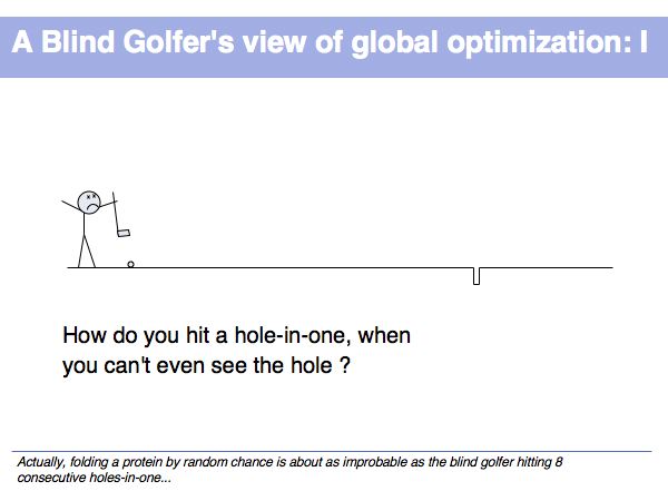
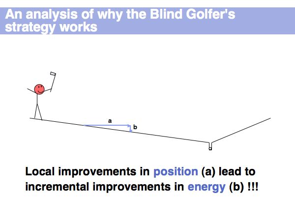
| + | A toy observation on an optimization problem of similar magnitude as the random folding of a protein... | ||
| + | ]] | ||
| − | |||
======Slide 005====== | ======Slide 005====== | ||
[[Image:L11_s005.jpg|frame|none|Lecture 11, Slide 005<br> | [[Image:L11_s005.jpg|frame|none|Lecture 11, Slide 005<br> | ||
| Line 86: | Line 96: | ||
======Slide 018====== | ======Slide 018====== | ||
[[Image:L11_s018.jpg|frame|none|Lecture 11, Slide 018<br> | [[Image:L11_s018.jpg|frame|none|Lecture 11, Slide 018<br> | ||
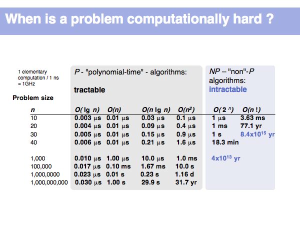
| + | Non-polynomial time-complexity problems are considered intractable, since even as the problem size ''''n'''' grows only modestly, the time requirements grow beyond all bounds and reasonable resources. A 1,000 element problem of ''O''(2<sup>''n''</sup>) complexity takes the age of the universe to compute. | ||
| + | ]] | ||
| − | |||
======Slide 019====== | ======Slide 019====== | ||
[[Image:L11_s019.jpg|frame|none|Lecture 11, Slide 019<br> | [[Image:L11_s019.jpg|frame|none|Lecture 11, Slide 019<br> | ||
| Line 110: | Line 121: | ||
======Slide 024====== | ======Slide 024====== | ||
[[Image:L11_s024.jpg|frame|none|Lecture 11, Slide 024<br> | [[Image:L11_s024.jpg|frame|none|Lecture 11, Slide 024<br> | ||
| + | Simulated annealing allows a system to be computationally moved out of situations where it is trapped in local minima, and to proceed towards a global minimum on a rough search landscape. | ||
| + | ]] | ||
| − | |||
======Slide 025====== | ======Slide 025====== | ||
[[Image:L11_s025.jpg|frame|none|Lecture 11, Slide 025<br> | [[Image:L11_s025.jpg|frame|none|Lecture 11, Slide 025<br> | ||
| + | A simulated annealing strategy (in pseudocode). | ||
| + | ]] | ||
| − | |||
======Slide 026====== | ======Slide 026====== | ||
[[Image:L11_s026.jpg|frame|none|Lecture 11, Slide 026<br> | [[Image:L11_s026.jpg|frame|none|Lecture 11, Slide 026<br> | ||
| + | Many believe that genetic algorithms - albeit interesting - rarely outperform simulated annealing. | ||
| + | ]] | ||
| − | |||
======Slide 027====== | ======Slide 027====== | ||
[[Image:L11_s027.jpg|frame|none|Lecture 11, Slide 027<br> | [[Image:L11_s027.jpg|frame|none|Lecture 11, Slide 027<br> | ||
| + | Natural proteins of course have evolved under the constraint of foldability. They may have avoided mutations that would expose them to the requirements of full, combinatorial optimization of their 3-D structure. | ||
| + | ]] | ||
| − | |||
======Slide 028====== | ======Slide 028====== | ||
[[Image:L11_s028.jpg|frame|none|Lecture 11, Slide 028<br> | [[Image:L11_s028.jpg|frame|none|Lecture 11, Slide 028<br> | ||
Latest revision as of 15:27, 1 September 2007
Update Warning! This page has not been revised yet for the 2007 Fall term. Some of the slides may be reused, but please consider the page as a whole out of date as long as this warning appears here.
(Previous lecture) ... (Next lecture)
Protein Structure Prediction
...
Add:
- Summary points
- Exercises
- Further reading
Lecture Slides
Slide 001
Slide 002
Slide 003
Slide 004
Slide 005
Slide 006
Slide 007
Slide 008
Slide 009
Slide 010
Slide 011
Slide 012
Slide 013
Slide 014
Slide 015
Slide 016
Slide 017
Slide 018

Lecture 11, Slide 018
Non-polynomial time-complexity problems are considered intractable, since even as the problem size 'n' grows only modestly, the time requirements grow beyond all bounds and reasonable resources. A 1,000 element problem of O(2n) complexity takes the age of the universe to compute.
Non-polynomial time-complexity problems are considered intractable, since even as the problem size 'n' grows only modestly, the time requirements grow beyond all bounds and reasonable resources. A 1,000 element problem of O(2n) complexity takes the age of the universe to compute.
